Complete Knapsack Theory Basics - Two-Dimensional DP Array

This problem doesn't have an exact match on LeetCode, but you can practice at the KamaCoder question 52 (opens new window), which has a similar problem statement.

Complete Knapsack Problem

You have N items and a knapsack that can carry a maximum weight of W. The weight of the i-th item is weight[i], and its value is value[i]. Each item is available in unlimited quantities (i.e., it can be placed in the knapsack multiple times). Find the maximum total value of items that can be placed in the knapsack.

The only difference between a complete knapsack and a 0/1 knapsack is that each type of item is available in unlimited quantities.

Similarly, LeetCode doesn't have a pure complete knapsack problem; they are applications that require transforming into a complete knapsack problem. Therefore, I will explain the theory and principles using a pure complete knapsack problem.

For the following explanation, I will use the data below as an example:

The knapsack's maximum weight is 4, and the items are:

	Weight	Value
Item 0	1	15
Item 1	3	20
Item 2	4	30

Each item is available in unlimited quantities!

What is the maximum value that the knapsack can carry?

If you haven't read the previous explanations on the 0/1 knapsack, make sure to carefully review the following two articles. The 0/1 knapsack is the foundation, and this article will not repeat those basics.

• Knapsack Theory 01 Knapsack-1 (opens new window)
• Knapsack Theory 01 Knapsack-2 (opens new window)

Let's analyze the complete knapsack problem's dynamic programming in five steps. To clearly understand the principles, we will first analyze a two-dimensional dp array:

1. Define the dp Array and the Index Meaning

dp[i][j] represents the maximum total value that can be achieved by considering items from index 0 to i, where each item can be used an unlimited number of times, given a knapsack capacity of j.

Many learners often wonder why we start by defining the dp array and what the thought process is like. I have explained this in detail in the section “Determine the dp Array and the Meaning of Indices” in the Knapsack Theory 01 Knapsack-1 (opens new window) article.

2. Determine the Recurrence Formula

Here are the basic details:

	Weight	Value
Item 0	1	15
Item 1	3	20
Item 2	4	30

To derive the recurrence formula, we must first clarify the directions from which we can infer dp[i][j].

Let's illustrate using the state dp[1][4]: (This is the same example as in the Knapsack Theory 01 Knapsack-1 (opens new window) article, but be sure to note the differences below.)

To determine dp[1][4], there are two scenarios:

1. Include item 1
2. Do not include item 1

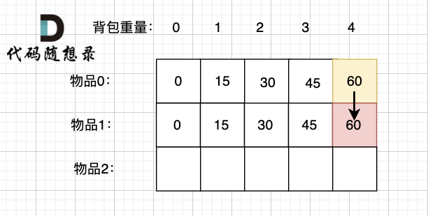
If item 1 is not included, then the maximum value with a knapsack capacity of 4 comes from only item 0, which is dp[0][4].

The deduction direction is shown in the diagram:

If item 1 is included, the knapsack must first leave room for the weight of item 1. Currently, the capacity is 4, and the weight of item 1 is 3, leaving a remaining capacity of 1 in the knapsack.

For a knapsack with capacity 1, considering only items 0 and 1, the maximum value is dp[1][1]. Note that this is different from the Knapsack Theory 01 Knapsack-1 (opens new window)!

In the Knapsack Theory 01 Knapsack-1 (opens new window), after leaving room for item 1, the capacity being 1 only considered the maximum value of item 0, which is dp[0][1]. Since every item in a 0/1 knapsack is only available once, if space for item 1 is left, item 1 will not be in the knapsack again!

However, in a complete knapsack, items can be placed an unlimited number of times. So even if item 1's space is left, item 1 could still be in the knapsack. Therefore, we still consider the maximum value of placing item 0 and item 1: dp[1][1], not dp[0][1].

Thus, the scenario for including item 1 is dp[1][1] + the value of item 1, as shown in the diagram:

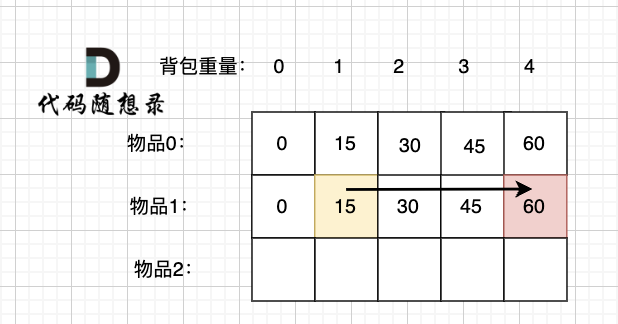
(Note the difference between the diagram above and the Knapsack Theory 01 Knapsack-1 (opens new window), which is crucial for understanding the complete knapsack)

The two scenarios, including item 1 and excluding item 1, leads us to take the maximum value (since we are seeking the maximum value).

dp[1][4] = max(dp[0][4], dp[1][1] + the value of item 1)

The above process can be abstracted as follows:

• Excluding item i: With knapsack capacity j, the maximum value without including item i is dp[i - 1][j].

• Including item i: After allocating space for item i's weight, the knapsack capacity is j - weight[i], dp[i][j - weight[i]] is the maximum value for a knapsack with capacity j - weight[i] without including item i. Therefore, dp[i][j - weight[i]] + value[i] (the value of item i) is the maximum value for including item i.

Recurrence formula: dp[i][j] = max(dp[i - 1][j], dp[i][j - weight[i]] + value[i]);

(Note the difference in the recurrence formula between the complete knapsack two-dimensional dp array and the 0/1 knapsack two-dimensional dp array. In the 0/1 knapsack, it is dp[i - 1][j - weight[i]] + value[i]))

3. Initialize the dp Array

The initialization must be consistent with the definition of the dp array; otherwise, it will become more chaotic when deriving the recurrence formula.

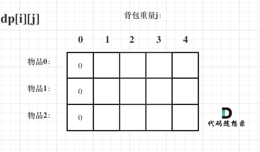
First, based on the definition of dp[i][j], if the knapsack capacity j is 0, then dp[i][0] must be 0, regardless of which items are selected, since the total value in the knapsack must be 0. As shown in the diagram:

Now, let's examine other cases.

The state transition formula dp[i][j] = max(dp[i - 1][j], dp[i][j - weight[i]] + value[i]); suggests that there is a direction where i is inferred from i-1, which means i = 0 must be initialized.

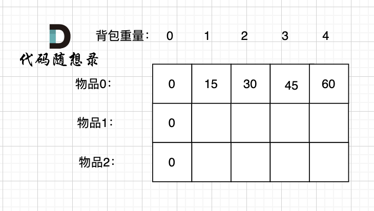
dp[0][j], i.e., considering only item 0 for various knapsack capacities, determines the maximum value that can be stored.

Clearly, when j < weight[0], dp[0][j] should be 0 because the knapsack capacity is less than the weight of item 0.

When j >= weight[0], if there's room for weight[0], we keep adding it since there are unlimited quantities of each item.

Such initialization in code looks like:

for (int i = 1; i < weight.size(); i++) {  // Of course, this step can be omitted if the dp array is initially set to 0, but many people haven't realized this point.
    dp[i][0] = 0;
}

// Iterate forward; if the item can be fit, keep adding item 0
for (int j = weight[0]; j <= bagWeight; j++)
    dp[0][j] = dp[0][j - weight[0]] + value[0];

(Notice the above initialization and the Knapsack Theory 01 Knapsack-1 (opens new window) differ in that items are unlimited)

At this point, the dp array initialization looks like the diagram below:

dp[0][j] and dp[i][0] have already been initialized, so how should other indices be initialized?

Actually, from the recursive formula: dp[i][j] = max(dp[i - 1][j], dp[i][j - weight[i]] + value[i]);, we can see that dp[i][j] is deduced from values above and to the left, so the initial value for other indices can be anything since they will be overwritten.

However, it is more convenient to initially set the entire dp array to 0.

Finally, the initialization code looks like this:

// Initialize dp
vector<vector<int>> dp(weight.size(), vector<int>(bagWeight + 1, 0));
for (int j = weight[0]; j <= bagWeight; j++) {
    dp[0][j] = dp[0][j - weight[0]] + value[0]; 
}

4. Determine the Order of Traversal

In the Knapsack Theory 01 Knapsack-1 (opens new window), we discussed that for a two-dimensional array in the 0/1 knapsack problem, you can iterate through either the items or the knapsack first.

Since both traversal orders provide the necessary values required by the recurrence formula for a two-dimensional dp array.

For details, see the Knapsack Theory 01 Knapsack-1 (opens new window) article's [Order of Traversal] section.

So, you could iterate over the items and then the knapsack:

for (int i = 1; i < n; i++) { // Traverse items
    for(int j = 0; j <= bagWeight; j++) { // Traverse knapsack capacity
        if (j < weight[i]) dp[i][j] = dp[i - 1][j];
        else dp[i][j] = max(dp[i - 1][j], dp[i][j - weight[i]] + value[i]);
    }
}

Or, you could iterate over the knapsack and then the items:

for(int j = 0; j <= bagWeight; j++) { // Traverse knapsack capacity
    for (int i = 1; i < n; i++) { // Traverse items
        if (j < weight[i]) dp[i][j] = dp[i - 1][j];
        else dp[i][j] = max(dp[i - 1][j], dp[i][j - weight[i]] + value[i]);
    }
}

5. Example to Derive the dp Array

Using the data in this article's example, the filled two-dimensional dp array looks like:

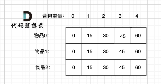
Since item 0 has the highest ratio of value to weight, and in the complete knapsack, there are unlimited quantities of each type of item, if item 0 has the highest cost-effectiveness, then item 0 should be prioritized.

Code for this Problem:

#include <iostream>
#include <vector>
using namespace std;

int main() {
    int n, bagWeight;
    int w, v;
    cin >> n >> bagWeight;
    vector<int> weight(n);
    vector<int> value(n);
    for (int i = 0; i < n; i++) {
        cin >> weight[i] >> value[i];
    }

    vector<vector<int>> dp(n, vector<int>(bagWeight + 1, 0));

    // Initialization
    for (int j = weight[0]; j <= bagWeight; j++)
        dp[0][j] = dp[0][j - weight[0]] + value[0];

    for (int i = 1; i < n; i++) { // Traverse items
        for(int j = 0; j <= bagWeight; j++) { // Traverse knapsack capacity
            if (j < weight[i]) dp[i][j] = dp[i - 1][j];
            else dp[i][j] = max(dp[i - 1][j], dp[i][j - weight[i]] + value[i]);
        }
    }

    cout << dp[n - 1][bagWeight] << endl;

    return 0;
}

For the one-dimensional dp array, see here: Complete Knapsack One-Dimensional dp Array Explanation

Versions in Other Languages

Java

import java.util.Scanner;

public class Main {
    public static void main(String[] args) {
        Scanner scanner = new Scanner(System.in);
        int n = scanner.nextInt();
        int bagWeight = scanner.nextInt();

        int[] weight = new int[n];
        int[] value = new int[n];

        for (int i = 0; i < n; i++) {
            weight[i] = scanner.nextInt();
            value[i] = scanner.nextInt();
        }

        int[][] dp = new int[n][bagWeight + 1];

        // Initialization
        for (int j = weight[0]; j <= bagWeight; j++) {
            dp[0][j] = dp[0][j - weight[0]] + value[0];
        }

        // Dynamic programming
        for (int i = 1; i < n; i++) {
            for (int j = 0; j <= bagWeight; j++) {
                if (j < weight[i]) {
                    dp[i][j] = dp[i - 1][j];
                } else {
                    dp[i][j] = Math.max(dp[i - 1][j], dp[i][j - weight[i]] + value[i]);
                }
            }
        }

        System.out.println(dp[n - 1][bagWeight]);
        scanner.close();
    }
}

Go

Python

def knapsack(n, bag_weight, weight, value):
    dp = [[0] * (bag_weight + 1) for _ in range(n)]

    # Initialization
    for j in range(weight[0], bag_weight + 1):
        dp[0][j] = dp[0][j - weight[0]] + value[0]

    # Dynamic programming
    for i in range(1, n):
        for j in range(bag_weight + 1):
            if j < weight[i]:
                dp[i][j] = dp[i - 1][j]
            else:
                dp[i][j] = max(dp[i - 1][j], dp[i][j - weight[i]] + value[i])

    return dp[n - 1][bag_weight]

# Input
n, bag_weight = map(int, input().split())
weight = []
value = []
for _ in range(n):
    w, v = map(int, input().split())
    weight.append(w)
    value.append(v)

# Output result
print(knapsack(n, bag_weight, weight, value))

JavaScript

const readline = require('readline').createInterface({
    input: process.stdin,
    output: process.stdout
});

let input = [];
readline.on('line', (line) => {
    input.push(line.trim());
});

readline.on('close', () => {
    // Parse the first line for n and v
    const [n, bagweight] = input[0].split(' ').map(Number);
    
    /// Parse the remaining n lines for weight and value
    const weight = [];
    const value = [];
    for (let i = 1; i <= n; i++) {
        const [wi, vi] = input[i].split(' ').map(Number);
        weight.push(wi);
        value.push(vi);
    }

    
    let dp = Array.from({ length: n }, () => Array(bagweight + 1).fill(0));

    for (let j = weight[0]; j <= bagweight; j++) {
        dp[0][j] = dp[0][j-weight[0]] + value[0];
    }

    for (let i = 1; i < n; i++) {
        for (let j = 0; j <= bagweight; j++) {
            if (j < weight[i]) {
                dp[i][j] = dp[i - 1][j];
            } else {
                dp[i][j] = Math.max(dp[i - 1][j], dp[i][j - weight[i]] + value[i]);
            }
        }
    }

    console.log(dp[n - 1][bagweight]);
});