20 tree structure diagrams, 14 curated backtracking problems, and 21 detailed articles on backtracking, progressing from simple to complex, making this the most comprehensive backtracking algorithm summary online!

Backtracking Summary

Backtracking Algorithm Fundamentals

In the Backtracking Algorithm Fundamentals (opens new window), we have already shared 21 days of backtracking algorithms. It is time to make a summary; this article requires a great deal of focus!

Regarding the fundamental theory of backtracking algorithms, I recorded a Bilibili video Learn Backtracking Algorithm in Depth (Theoretical Part) (opens new window). If you're not familiar with backtracking algorithms, you might want to check it out.

In What You Should Know About Backtracking Algorithms! (opens new window), we provide an in-depth explanation of the fundamental knowledge of backtracking algorithms. Unlike textbook explanations, this introduction focuses on efficiency, problems to solve, and templates that are practically useful during problem-solving!

Backtracking is a byproduct of recursion; wherever there is recursion, there is backtracking. Therefore, backtracking is often mixed with binary tree traversal and depth-first search because both use recursion.

Backtracking is essentially brute-force search and is not an efficient algorithm, with most cases involving pruning.

Backtracking can solve the following types of problems:

• Combination problems: Finding k number sets out of N numbers following certain rules
• Permutation problems: Determining the number of permutation ways for N numbers following certain rules
• Partitioning problems: Finding the number of ways a string can be partitioned following certain rules
• Subset problems: Finding subsets of an N-element set that meet certain conditions
• Board problems: Such as N-Queens and Sudoku solving

I've followed this sequence to explain backtracking algorithms to ensure thorough understanding by gradual steps.

Backtracking can be challenging to understand, but visualizing backtracking as a graph makes it easier comprehensible. For every backtracking problem discussed later, I will abstract the traversal process as a tree structure to aid understanding.

In What You Should Know About Backtracking Algorithms! (opens new window), I break down backtracking algorithms using the backtracking three-step process and provide a template for backtracking:

void backtracking(parameters) {
    if (termination condition) {
        store result;
        return;
    }

    for (choices: elements in the current level set (the number of child nodes in a tree node is the size of the set)) {
        process node;
        backtracking(path, choices list); // recursion
        backtrack, undo process result
    }
}

This template proves to accompany the entire backtracking series!

Combination Problems

Combination Problems

In 0077. Combinations (opens new window), we start using backtracking to solve the first problem: combination problems.

In the article, I begin by listing examples of k layers of for loops, then derive why backtracking is necessary even though it's similar to brute-force solutions!

By this time, everyone should deeply appreciate the charm of backtracking, using recursion to control the number of for loop nests!

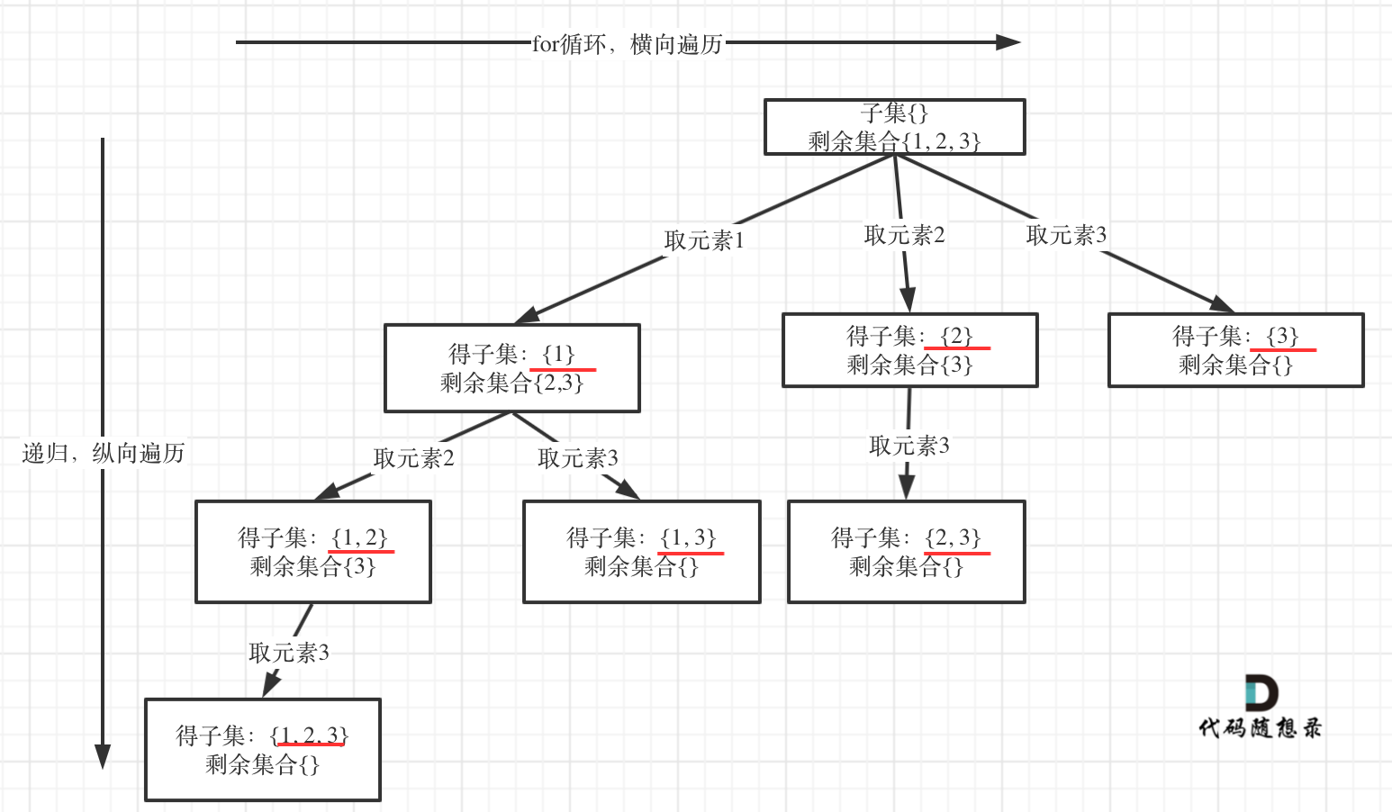
In this problem, I've abstracted the backtracking problem into a tree structure, as shown below:

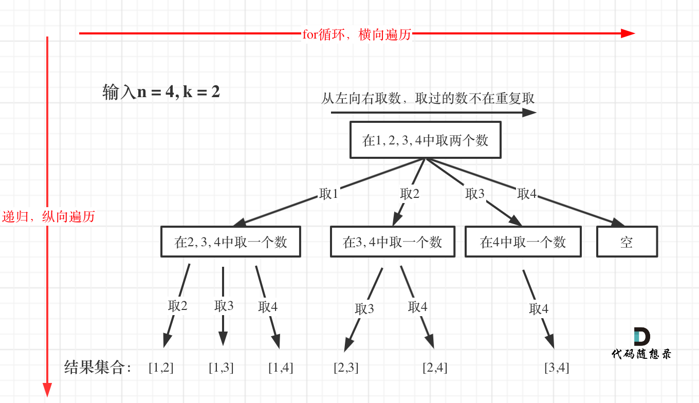
You can intuitively see the search process: For loop traverses horizontally, recursion traverses vertically, and the result set is continuously adjusted by backtracking. This concept is consistent throughout the backtracking series and is the pattern I discovered after solving many backtracking problems.

When it comes to the overall framework of backtracking, online articles on this topic usually do not explain it clearly; most seem to rely on seemingly arbitrary code, without explaining the logic behind the implementation.

Therefore, friends who've just started learning backtracking are off to an excellent start!

Optimizing backtracking algorithms primarily involves pruning, which I explained in 0077. Combination Optimization (opens new window) by optimizing the backtracking code through pruning. The tree structure is as follows:

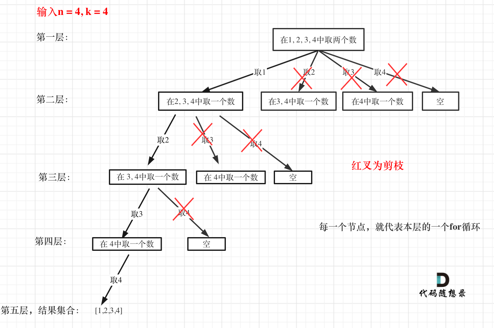
You can clearly see where the pruning occurs.

0077. Combination Optimization (opens new window) highlights the essence of pruning: In a for loop, a starting point range must exist. If the elements from this starting point to the end of the set do not provide the required k elements as per the problem requirements, further searching is unnecessary.

Pruning using the for loop is a common backtracking optimization strategy! You'll frequently encounter it in later problems.

Combination Sum

Combination Sum (I)

In 0216. Combination Sum III (opens new window), it's similar to 0077. Combinations (opens new window) with an additional constraint on the sum of elements.

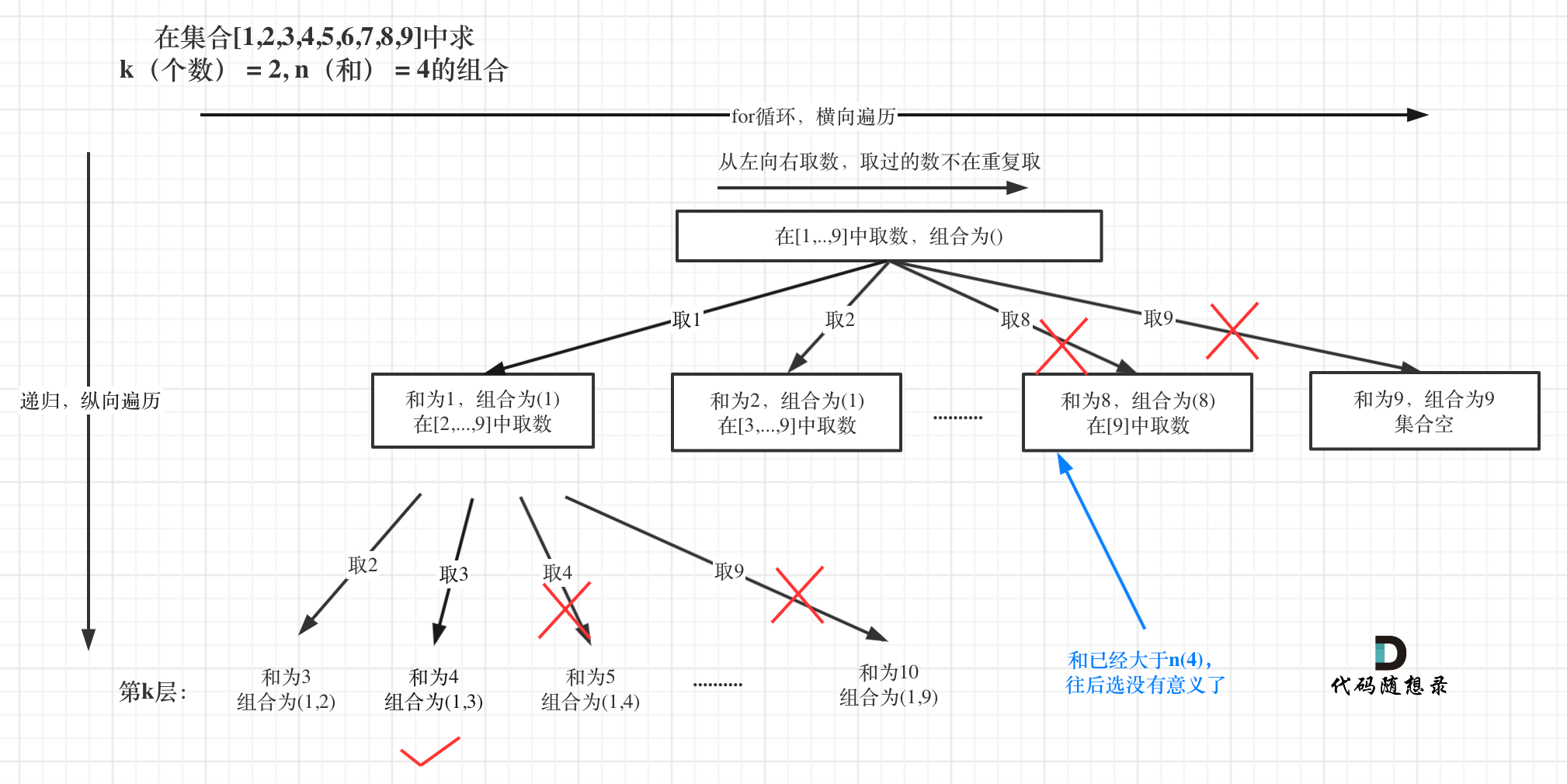
The tree structure is as follows:

The overall approach remains the same, but the pruning in this problem is simpler. That is: Once the sum of selected elements exceeds n (the required sum in the problem), further traversal is meaningless, and it should be pruned, as shown:

In this problem, pruning similar to the one mentioned in 0077. Combination Optimization (opens new window) can be used, where a range limit is applied to the starting point selected in the for loop.

Therefore, the pruning code can add a constraint like i <= 9 - (k - path.size()) + 1 in the for loop!

Combination Sum (II)

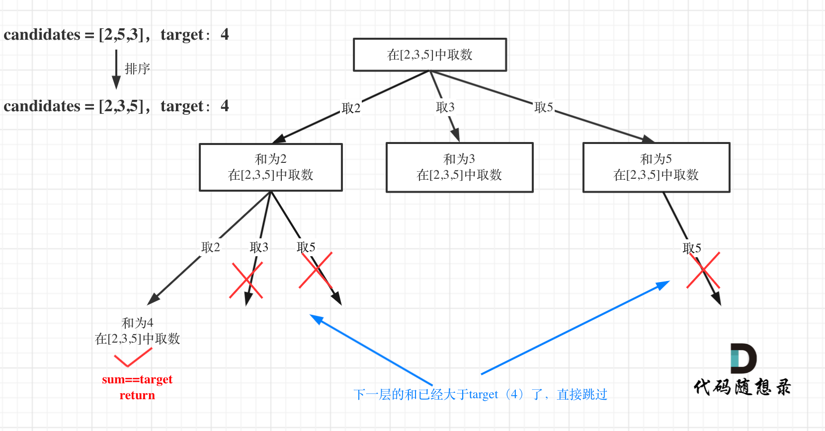
In 0039. Combination Sum (opens new window), a combination sum problem is discussed, differing from 0077. Combinations (opens new window) and 0216. Combination Sum III (opens new window) in that this problem does not require a specific quantity and can have an infinite number of repetitions, albeit with a limit on the sum, which indirectly limits the number.

Many people hastily remove startIndex upon seeing possible repeated selections.

When is startIndex needed for combination problems?

I gave examples; if it's a single set looking for combinations, then startIndex is necessary, as in 0077. Combinations (opens new window) and 0216. Combination Sum III (opens new window).

If it's multiple independent sets for combinations, then startIndex is not needed, as in 0017. Letter Combinations of a Phone Number (opens new window).

Note that this applies only to combination problems; permutation problems require a different analytical approach.

The tree structure is as follows:

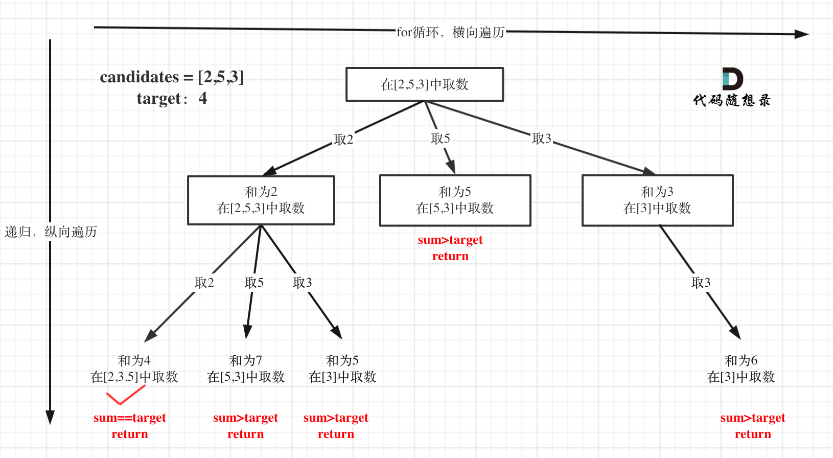
Finally, an additional optimization is provided for pruning in this problem, as follows:

for (int i = startIndex; i < candidates.size() && sum + candidates[i] <= target; i++)

The optimized tree structure is as follows:

Combination Sum (III)

In 0040. Combination Sum II (opens new window), the set elements can repeat, but the solution set must not contain duplicate combinations.

Thus, the challenge lies primarily in dealing with duplicates.

The duplicates issue in this problem is notoriously complex. Online solutions often briefly mention "removing duplicates," but rarely offer a clear explanation; code is usually just presented.

To clarify the duplicates issue, I've coined two phrases, "pruning branches" and "pruning levels".

It is known that combination problems can be abstracted into tree structures, where "used" can be understood in two dimensions on this tree structure: one is "used" in the same tree branch, and the other is "used" at the same tree level. Failing to understand "used" from these two dimensions is the root cause of confusion regarding deduplication.

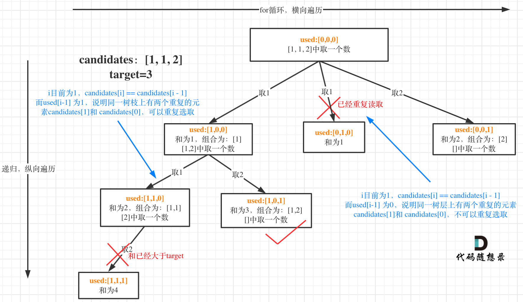
In the diagram, I mark changes to used in orange. It can be seen that when candidates[i] == candidates[i - 1], the following applies:

• used[i - 1] == true, indicating candidates[i - 1] has been used on the same tree branch.
• used[i - 1] == false, indicating candidates[i - 1] has been used at the same tree level.

This pruning logic is very abstract, and most online solutions fail to clearly explain it. If you have previously pondered this issue or solved this problem, this section should bring much clarity!

The same deduplication principles apply to permutation and subset problems.

Combinations of Multiple Sets

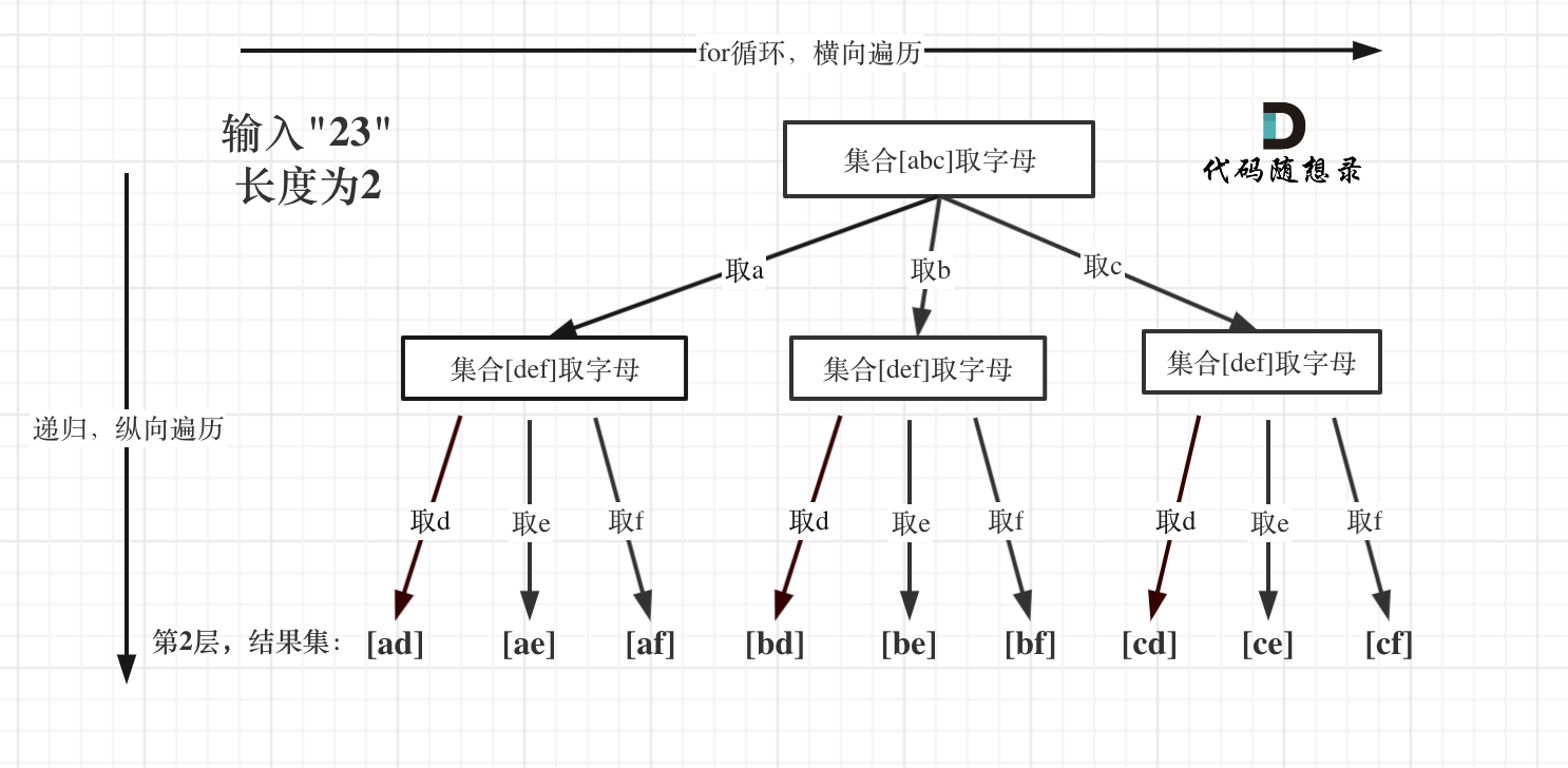
In 0017. Letter Combinations of a Phone Number (opens new window), we begin using combinations of multiple sets; it is another familiar template problem, but with some nuances.

For instance, in the for loop, it does not start from startIndex as seen in 0077. Combinations (opens new window) and 0216. Combination Sum III (opens new window).

That's because the problem involves combining elements from different sets, unlike 0077. Combinations (opens new window) and 0216. Combination Sum III (opens new window), which deal with combinations within a single set!

The tree structure is as follows:

In live interviews, always pay attention to various input anomalies, such as input with 1 * # keypresses.

Although not difficult, this problem involves subtle details and should be carefully considered.

Partitioning Problems

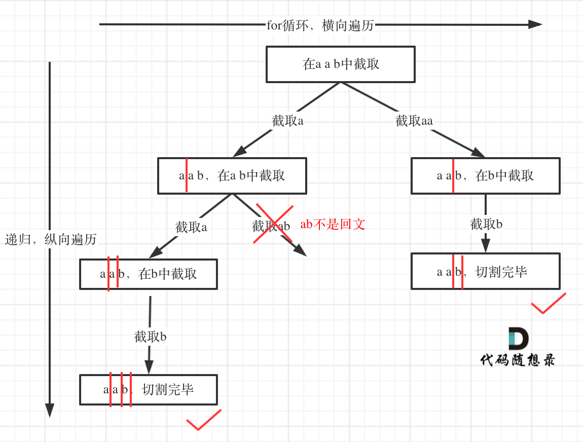
In 0131. Palindrome Partitioning (opens new window), we start discussing partitioning problems, and although the final code appears to follow a template, understanding and adapting it to this template can be challenging.

Here are some noted difficulties:

• Partitioning problems are similar to combination problems
• How to simulate cutting lines
• How to define termination in recursion for partitioning problems
• How to extract substrings during recursive loops
• How to determine palindromes

If you think of solving partitioning problems using a combination problem approach, you've completed most of the problem-solving process. Then, you can adapt this template to your work.

However, how to simulate cutting lines, when to terminate, how to extract substrings, and finally determining palindromes, are all challenging to figure out. Knowing how to determine palindromes is the simplest part.

Therefore, this problem should be considered a hard problem.

Alongside these challenges, one aspect: once partitioned, the same place cannot be partitioned again, so pass i + 1 into the recursion function.

The tree structure is as follows:

Subset Problems

Subset Problem (I)

In 0078. Subsets (opens new window), subset problems are discussed. Within tree structures, subset problems involve collecting results from all nodes, while combination problems only collect leaf node results.

As shown:

Recognizing this essence, today's problem becomes a template.

An end condition is unnecessary because startIndex >= nums.size() will naturally end the current level for loop, and we aim to traverse the entire tree.

Some worry that not writing an end condition might result in endless recursion, but it won't because each recursion starts from i + 1.

If adding an end condition, note: result.push_back(path); must be above the end condition, like this:

result.push_back(path); // Collect subsets, placed above termination addition to prevent result omission
if (startIndex >= nums.size()) { // Termination condition not needed
    return;
}

Subset Problem (II)

In 0090. Subsets II (opens new window), deduplication begins for subset problems.

This problem is an extension of 0078. Subsets (opens new window) with deduplication, discussed before in 0040. Combination Sum II (opens new window), using the same logic.

The tree structure is as follows:

Non-decreasing Subsequences

In 0491. Non-decreasing Subsequences (opens new window), glimpses of the subset issue are evident throughout, with traps to consider thoughtfully!

The tree structure is as follows:

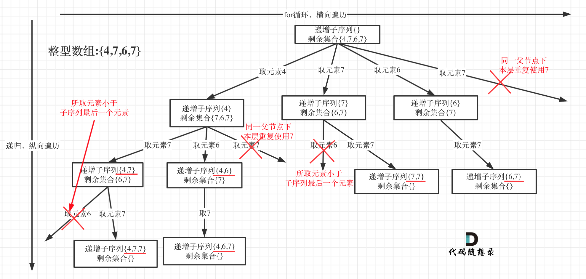
Many often confuse this question with 0090. Subsets II (opens new window).

Set can be used to deduplicate in the same parent node layer, which is feasible in 0090. Subsets II (opens new window), but sorting is crucial for deduplication, why?

I'll draw a picture using an unsorted set {2, 1, 2, 2} as an example:

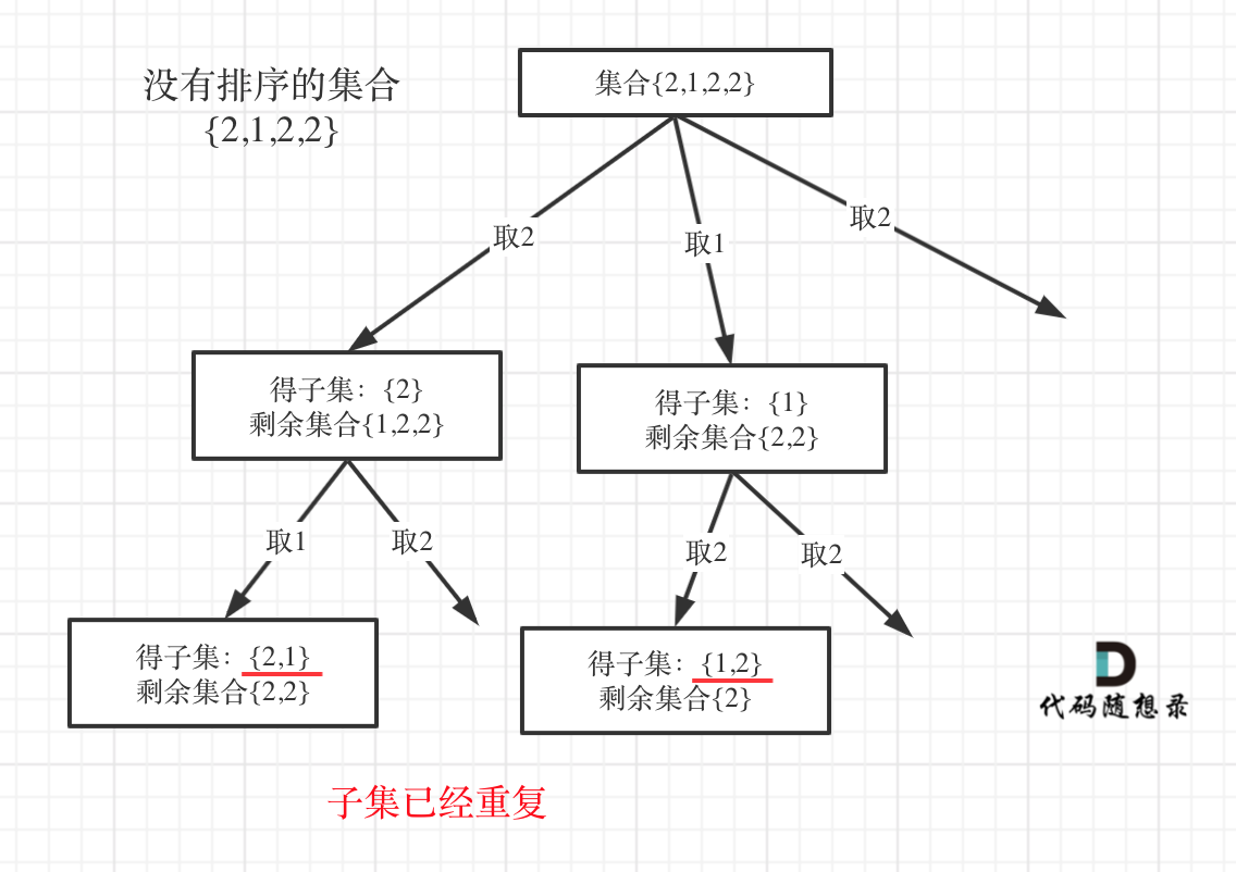
I believe this picture explains more than thousands of words.

Permutation Problems

Permutation Problem (I)

0046. Permutations (opens new window) is different too.

Permutations are ordered; [1,2] and [2,1] are two sets, differing from subsets and combinations analyzed before.

It can be noted that element 1 is used in [1,2] and needs to be reused in [2,1], so startIndex is unnecessary for permutations.

As shown:

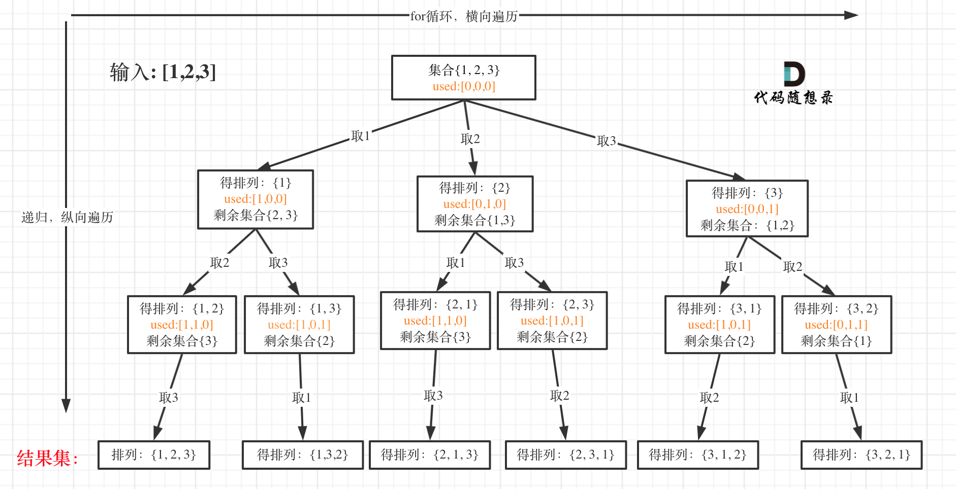
With an appreciation for learning the distinction of permutation problems:

• Each layer starts searching from 0, unlike startIndex
• Needs used array to record elements included in path

Permutation Problem (II)

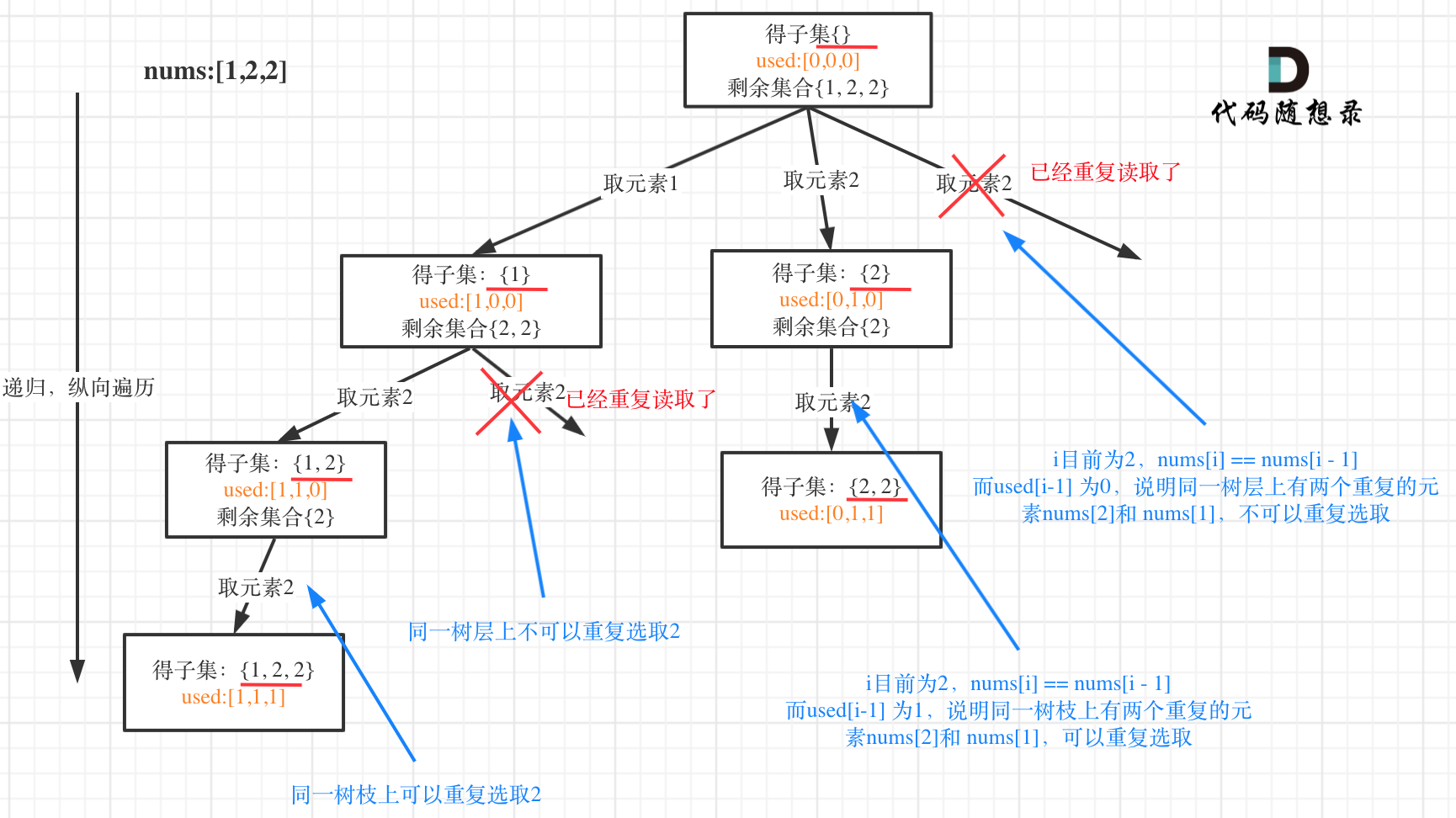
Deduplication for permutation problems starts in 0047. Permutations II (opens new window), with revisited emphasis on "pruning branches" and "pruning levels."

The tree structure is as follows:

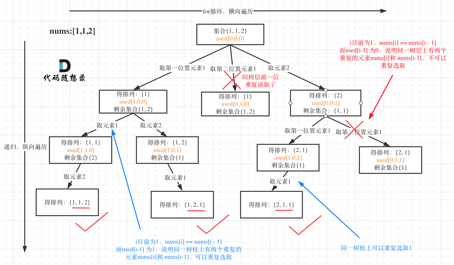
Interestingly, this question allows for used[i - 1] == false or used[i - 1] == true!

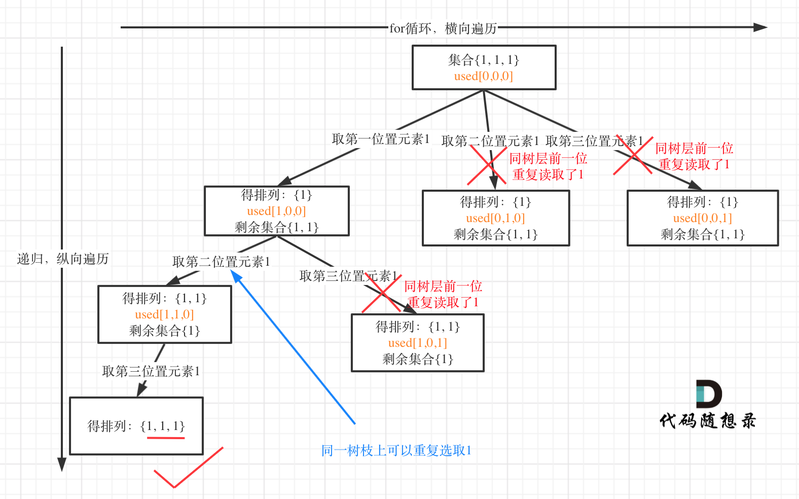
A practical example: Input: [1,1,1].

Tree level deduplication (used[i - 1] == false) structure:

Tree branch deduplication (used[i - 1] == true) structure:

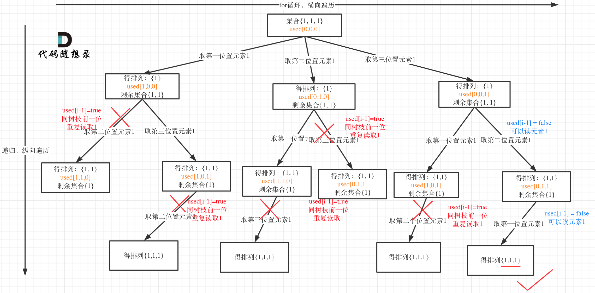
It is evident that using (used[i - 1] == false) for tree level deduplication is less computationally intensive!

The used array records elements in the path while providing deduplication benefits.

Deduplication Issues

Previously, I consistently used the used array for deduplication; using set also achieves deduplication!

In Backtracking Algorithm for Deduplication - Alternative Approach (opens new window), I provided solutions and code illustrating deduplication via set for subsets, combinations, and permutations, while correcting common mistakes made by peers.

In-depth discussions on the performance discrepancy between used array and set removal:

Deduplication using set appears considerably slower than the used array, visibly noticeable when submitting on LeetCode.

The performance difference is analyzed in detail as seen in 0491. Non-decreasing Subsequences (opens new window). The key reason is the high computational cost of frequent insert operations on the unordered_set for hash mapping (converting keys to unique hash values via hash functions) and its underlying table symbol expansions.

The used array artfully avoids this time complexity burden!

Using set causes computational overhead not only in time complexity but also in space complexity;

In Weekly Summary! (Backtracking Series III) Continued (opens new window), it has been analyzed, showing space complexity for combinations, subsets, and permutations is O(n), but using set increases space complexity to O(n^2), because each recursion level has its set.

Some might wonder if the used array isn't also consuming O(n) space?

The used array serves as a global variable, shared across all levels, resulting in a complexity of O(n + n), ultimately remaining O(n).

Reconstruct Itinerary (Graph Theory Extension)

It was stated that recursion implies backtracking, and depth-first search uses recursion, so often they accompany each other.

In 0332. Reconstruct Itinerary (opens new window), it is a depth-first search (DFS) problem, yet it is expounded via backtracking thinking, broadening the conception that backtracking can be flexible!

With input: [["JFK", "KUL"], ["JFK", "NRT"], ["NRT", "JFK"], it abstracts into a tree structure as follows:

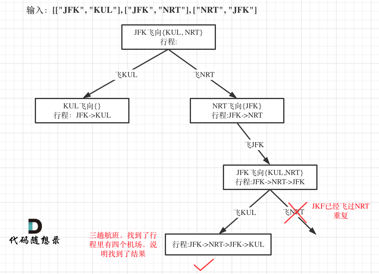
This problem is arguably a hard one, detailed challenges are outlined in the article.

Simple backtracking search (DFS) isn't difficult; the complexity lies in choosing and using data structures!

The problem, essentially a DFS, is explicitly explained using a backtracking thought process, broadening the range of backtracking's application in problem-solving.

Chessboard Problems

N-Queens

In 0051. N-Queens (opens new window), the legendary N-Queens problem finally appears.

For a 3 * 3 board, the search process can be abstracted as follows:

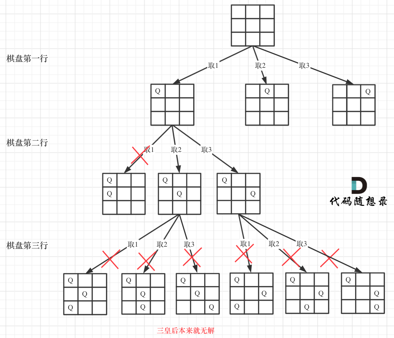
From the diagram, the board's height is the tree's height, and the board's width equates to a tree node's width.

Consequently, using the constraints of queens, the backtracking search of this tree can be conducted. Once the tree's leaf node is reached, the queens' correct placements are determined.

Those unfamiliar with the N-Queens problem might feel it is intractable. Recognizing backtracking is necessary, yet uncertain how to search.

By explaining the board width equates to for loop length and recursion depth equals board height, a definitive framework fits into the backtracking template.

It's no longer perceived as difficult. The legend ceases to remain a legend.

Sudoku Solver

In 0037. Sudoku Solver (opens new window), tackling backtracking's last summit.

Sudoku solving is perhaps the most challenging chessboard problem, slightly more complex than N-Queens, yet once the concept of "two-dimensional recursion" is understood, it becomes manageable.

As readers have studied problems such as 0077. Combinations (opens new window), 0131. Palindrome Partitioning (opens new window), 0078. Subsets (opens new window), 0046. Permutations (opens new window), as well as 0051. N-Queens (opens new window), these are all "one-dimensional recursion."

N-Queens (opens new window) requires placing one queen per row and column, thus involving a singular loop where recursion tackles columns, aligning the respective positions of any queen singularly.

This problem differs wherein every position on the Sudoku board requires a number and validating legality, creating a tree structure both wide and deep in Sudoku solving, exceeding N-Queens.

Limited space presents part of the tree:

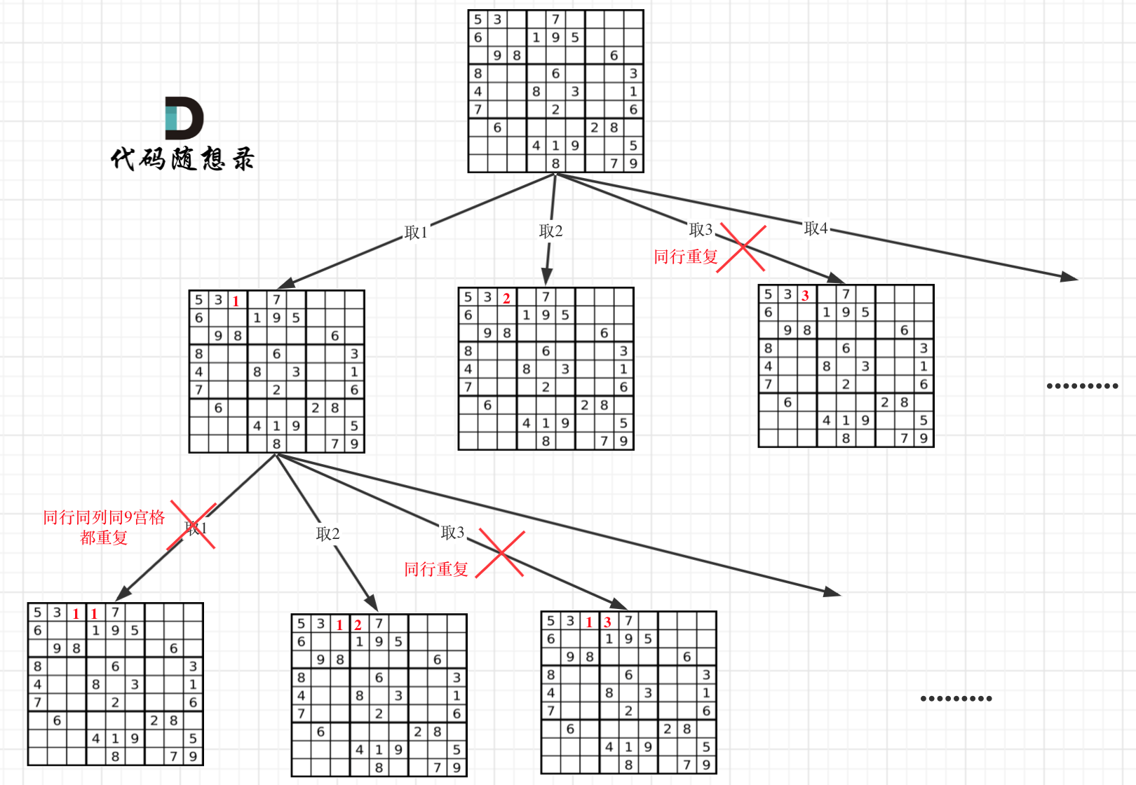
Sudoku solving is extraordinarily challenging. When stuck in one-dimensional recursion logic, such problems could lead to significant frustration.

Therefore, I introduced "two-dimensional recursion," a novel concept, to explore problem-solving in 0037. Sudoku Solver (opens new window).

Upon contemplation, even the code won't seem daunting; grasping two-dimensional recursion alone is the complexity.

Subsequently, solving Sudoku—historically complex—is achieved.

Performance Analysis

In online discussions, the complexities of backtracking algorithms yield mixed perspectives. Many books on interviews and algorithms avoid this, leaving an ambiguous edge in understanding.

I want to express personal understanding here, maintained open to community dialogue, invitations welcome!

When including the system stack space during space complexity evaluation:

Subset Problem Analysis:

• Time Complexity: O(2^n), each element's state is evidently limited to being considered or not, settling complexity at O(2^n).
• Space Complexity: O(n), recursion depth is n, occupying O(n) space in the system stack. Each layer of recursion uses constant space, and variables result and path are global, bearing no new memory allocation. Final space complexity remains O(n).

Permutation Problem Analysis:

• Time Complexity: O(n!), clearly visible from permutation trees, each layer has n nodes; second layer splits to n-1 branches and so forth down to leaf nodes forming n * (n-1) * ... * 1 = n!.
• Space Complexity: O(n), similar to subset problems.

Combination Problem Analysis:

• Time Complexity: O(2^n), combination problems are essentially subset problems. Hence, at worst, the complexity won't surpass subset problems.
• Space Complexity: O(n), relationally identical to subsets.

N-Queens Problem Analysis:

• Time Complexity: O(n!), intuition suggests O(n^n) from tree perspectives. Nonetheless, due to pruning from queen restrictions, the worst-case complexity is O(n!), reflecting n * (n-1) * ... * 1 = n!.
• Space Complexity: O(n), aligned with subsets.

Sudoku Solver Problem Analysis:

• Time Complexity: O(9^m), with m denoting count of '.'.
• Space Complexity: O(n^2), recursion depth at n^2.

Backtracking algorithm complexity often exhibits exponential behavior, a succinct overview!

Conclusion

Through 21 days in the “Programmer Thinking Record” (opens new window), writing 14 classic problem analyses, 20 tree diagrams, and 21 detailed articles on the backtracking algorithm, from sets to partitioning, subsets to permutations, chessboard problems, and finally complexity analysis. With this conclusion, a wrap-up is necessary.

In each aria, a comparative approach was adopted through explanations, ensuring comprehensive clarity across facets.

Exemplifying inquiries like:

• How to understand the backtracking search process?
• When and why startIndex is needed?
• How deduplication works? What are "pruning branches" and "pruning levels"?
• What are the methods for deduplication?
• How to perceive two-dimensional recursion?

These key questions elude comprehensible articles online, directly targeting the essence of backtracking.

Persistent dedication granted by fellow readers couldn't leave them without a profound understanding of the backtracking algorithm.

With the backtracking series, a formal cessation is upon us.

Readers may reflect on these 21 days, daily card markings and exchanges in discussion groups, unwittingly their growth became evident.

Thanks convincingly to the persevering endeavors of the readers, it fuels my continuous writing, it emboldened, proving the meaningful significance behind it.

The backtracking collection, consolidated into one diagram:

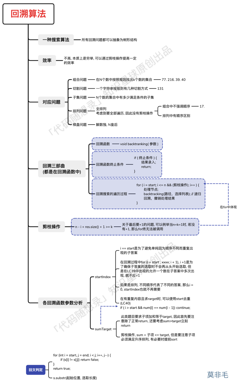
This diagram is contributed by a KStar member: Mo Fei Mao (opens new window), summed extraordinarily well and shared for everyone.