# 743. Network Delay Time

https://leetcode.com/problems/network-delay-time/description/

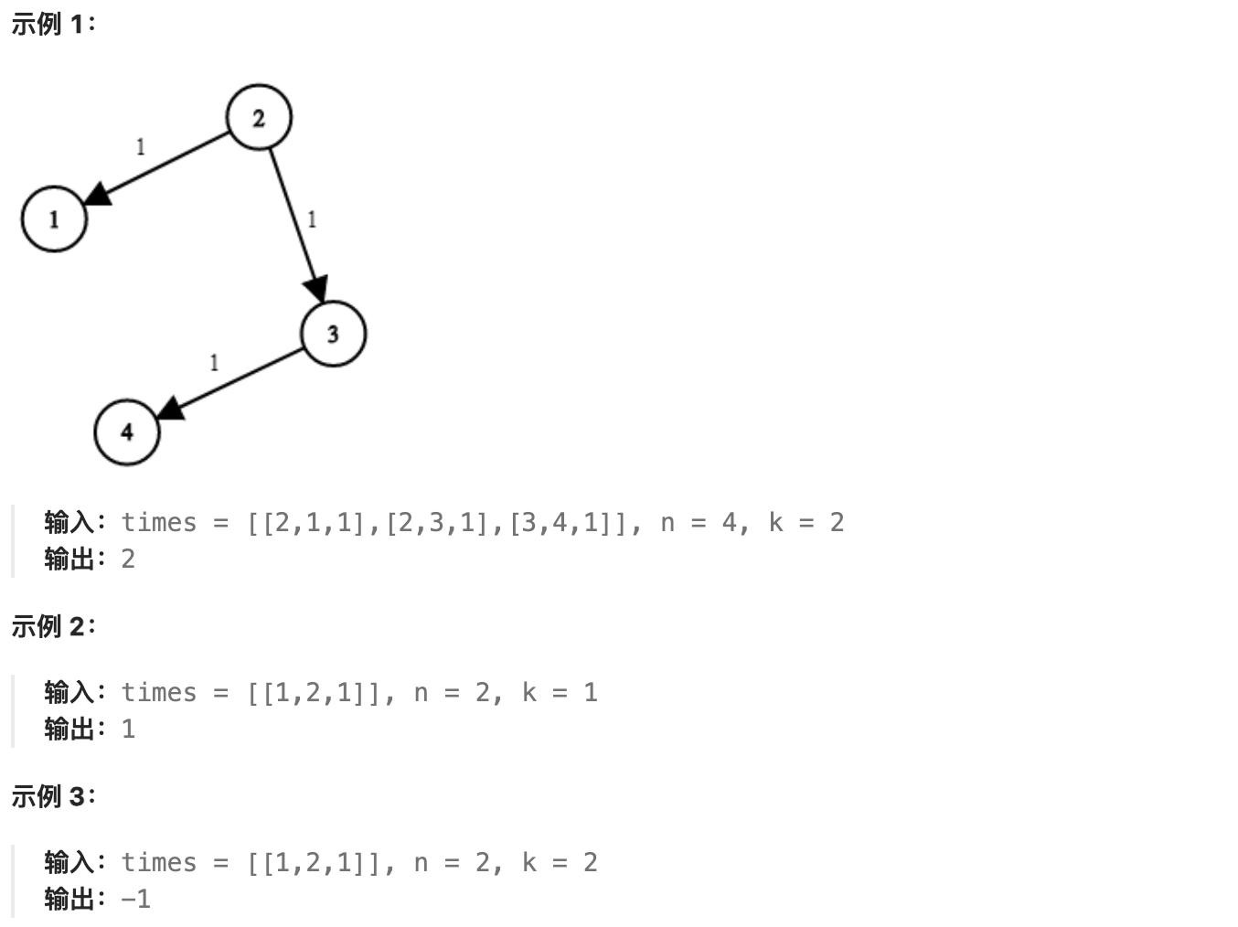
There are `n` network nodes, labeled from 1 to `n`.

You are given a list `times`, which represents the transmission time of a signal through directed edges. `times[i] = (ui, vi, wi)`, where `ui` is the source node, `vi` is the target node, and `wi` is the time taken for the signal to be transmitted from the source node to the target node.

Now, a signal is sent from a certain node `K`. How long will it take for all nodes to receive the signal? If it is impossible for all nodes to receive the signal, return `-1`.

![Example Image](https://file1.kamacoder.com/i/algo/20240229104105.png)

**Constraints:**

- 1 <= k <= n <= 100
- 1 <= times.length <= 6000
- times[i].length == 3
- 1 <= ui, vi <= n
- ui != vi
- 0 <= wi <= 100
- All pairs `(ui, vi)` are unique (i.e., no duplicate edges)

# Detailed Explanation of Dijkstra's Algorithm

This problem is essentially about finding the shortest path, which is a classic problem in graph theory: given a directed graph, a start vertex, and an end vertex, find the shortest path from the start to the end.

Let's dive into the details of Dijkstra's algorithm within the shortest path algorithms.

**Dijkstra's Algorithm**: An algorithm to find the shortest paths from a start node to all other nodes in a graph with non-negative edge weights.

Two key points to note:

- Dijkstra's algorithm can find the shortest paths from the start node to all nodes.
- Edge weights cannot be negative.

(These two points will be elaborated later.)

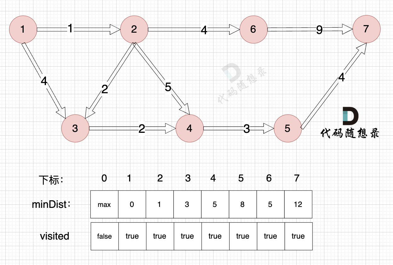
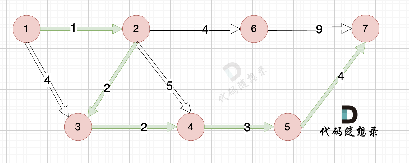
As shown in the example graph:

![Graph Example](https://file1.kamacoder.com/i/algo/20240125162647.png)

The shortest path from the start node (node 1) to the end node (node 7) is highlighted with green lines.

The total weight of the shortest path is 12.

In fact, the thought process behind Dijkstra's algorithm is very similar to Prim's algorithm. If you have understood Prim's algorithm well, Dijkstra's algorithm will be relatively easy to grasp. (This is also why I wanted to explain Prim before Dijkstra.)

Dijkstra's algorithm is greedy, constantly looking for the unvisited node closest to the source node.

Here are the **three steps of Dijkstra's algorithm**:

1. Step one: Choose the unvisited node closest to the start node.
2. Step two: Mark this closest node as visited.
3. Step three: Update the distance to the source node for unvisited nodes (update the `minDist` array).

You might notice that this is strikingly similar to Prim's algorithm.

In Dijkstra's algorithm, there is a crucial array named `minDist`.

**The `minDist` array is used to record the minimum distance from each node to the source node.**

Understanding this is important and is at the core of understanding Dijkstra's algorithm.

You might be a little confused now, not knowing what it means.

Don't worry, it's just an introduction now. It will help you understand the explanation later.

Let's look at a visual representation of how Dijkstra's works using the example in this problem: (The following is a thought process for the basic version of Dijkstra.)

(The nodes in the example are labeled starting from 1, so to avoid confusion, I will also start the `minDist` array from index 1. Index 0 will be unused, so that indices correspond to node numbers, avoiding confusion.)

## Basic Version of Dijkstra

### Simulation Process

-----------

0. Initialization

Initialize the values in the `minDist` array to the maximum integer value.

Here, I want to emphasize the meaning of the `minDist` array: it records the shortest distance from the source to all nodes. Initialization should be maximum so it can be updated upon finding a shorter path.

![Initialization](https://file1.kamacoder.com/i/algo/20240130115306.png)

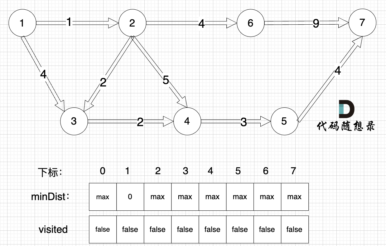
(In the diagram, `max` stands for default values, and node 0 is not processed. All calculations start from index 1 so that indices and node values align for easy understanding, avoiding confusion.)

The distance from the source (node 1) to itself is 0, so `minDist[1] = 0`.

At this point, all nodes are unvisited, so the `visited` array is all 0s.

---------------

Below is the Dijkstra Three Steps:

1. Choose the unvisited node closest to the start node.

Node 1 is closest to the start, with a distance of 0, and is unvisited.

2. Mark this node as visited.

Mark the source node as visited.

3. Update the distance to the source node for unvisited nodes (update the `minDist` array), as shown:

![Step 1](https://file1.kamacoder.com/i/algo/20240130115421.png)

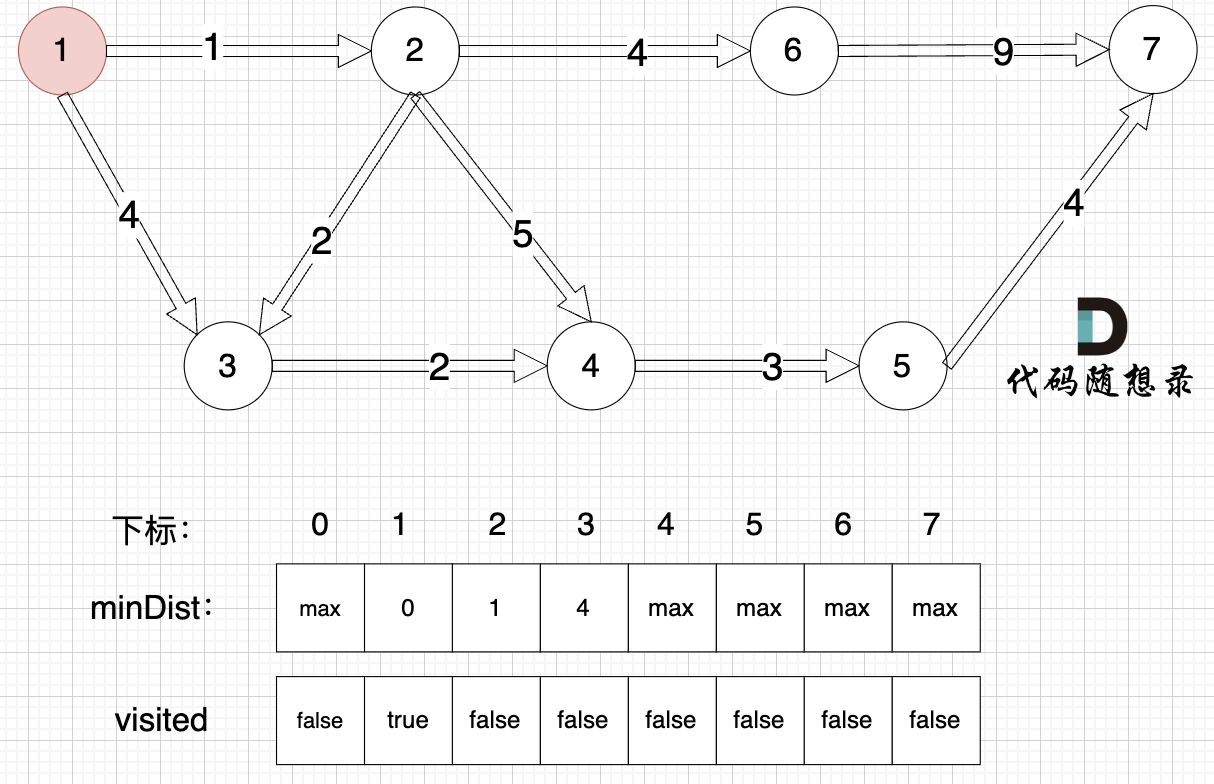
Update the `minDist` array, i.e., distance from the source (node 1) to nodes 2 and 3:

- The shortest distance from the source to node 2 is 1, which is less than the previous value of `minDist[2]`, which was `max`, so update `minDist[2] = 1`.
- The shortest distance from the source to node 3 is 4, which is less than the previous value of `minDist[3]`, which was `max`, so update `minDist[3] = 4`.

Some may ask why compare with `minDist[2]`?

Re-emphasizing, `minDist[2]` represents the shortest distance from the source to node 2, and the shortest distance from the source to node 2 is currently 1, which is less than the default value `max`, so update. The update for `minDist[3]` follows the same reasoning.

-------------

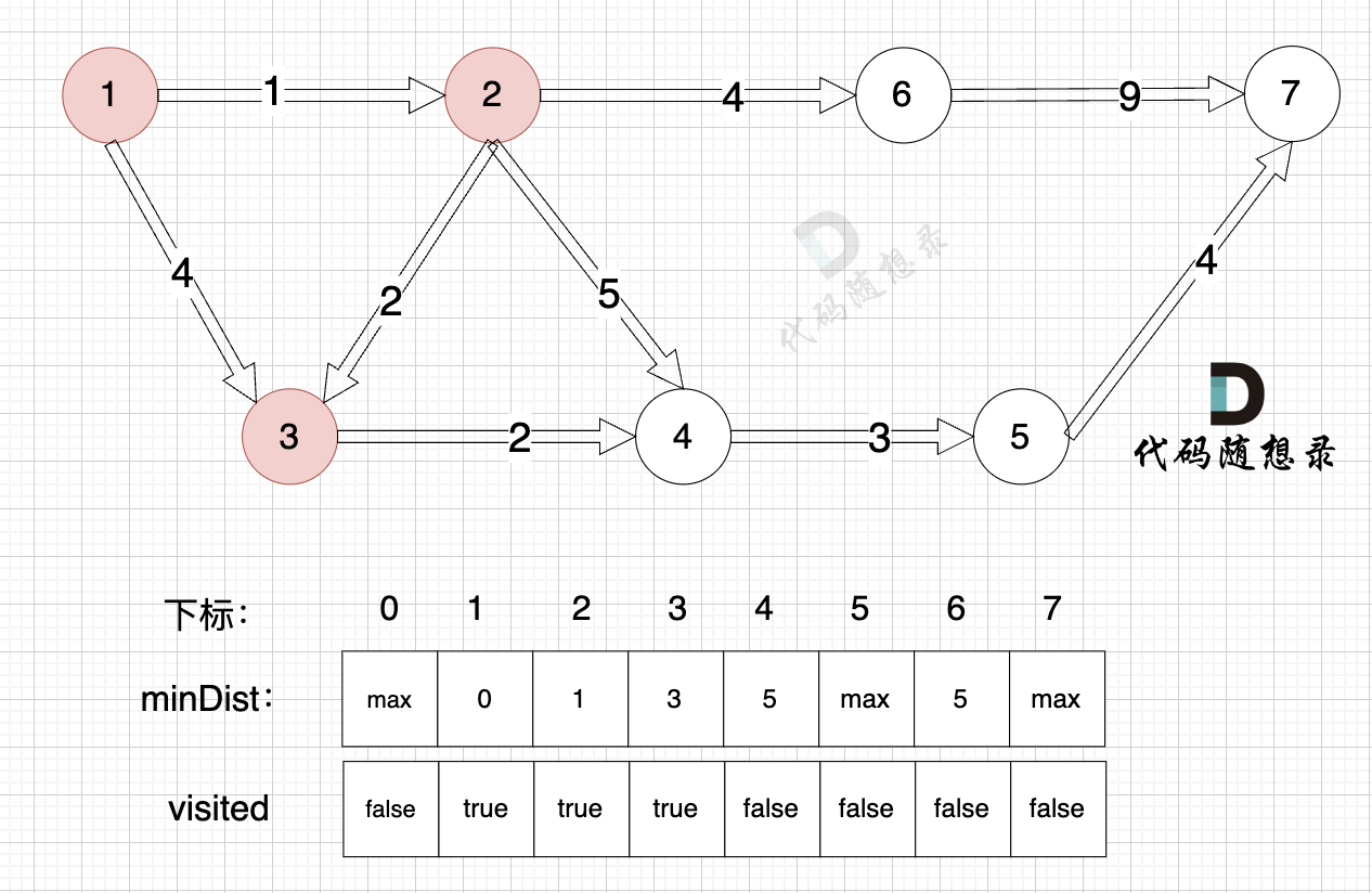
1. Choose the unvisited node closest to the start node.

Of the unvisited nodes, node 2 is closest to the source, so node 2 is chosen.

2. Mark this node as visited.

Mark node 2 as visited.

3. Update the distance to the source node for unvisited nodes (update the `minDist` array), as shown:

![Step 2](https://file1.kamacoder.com/i/algo/20240130121240.png)

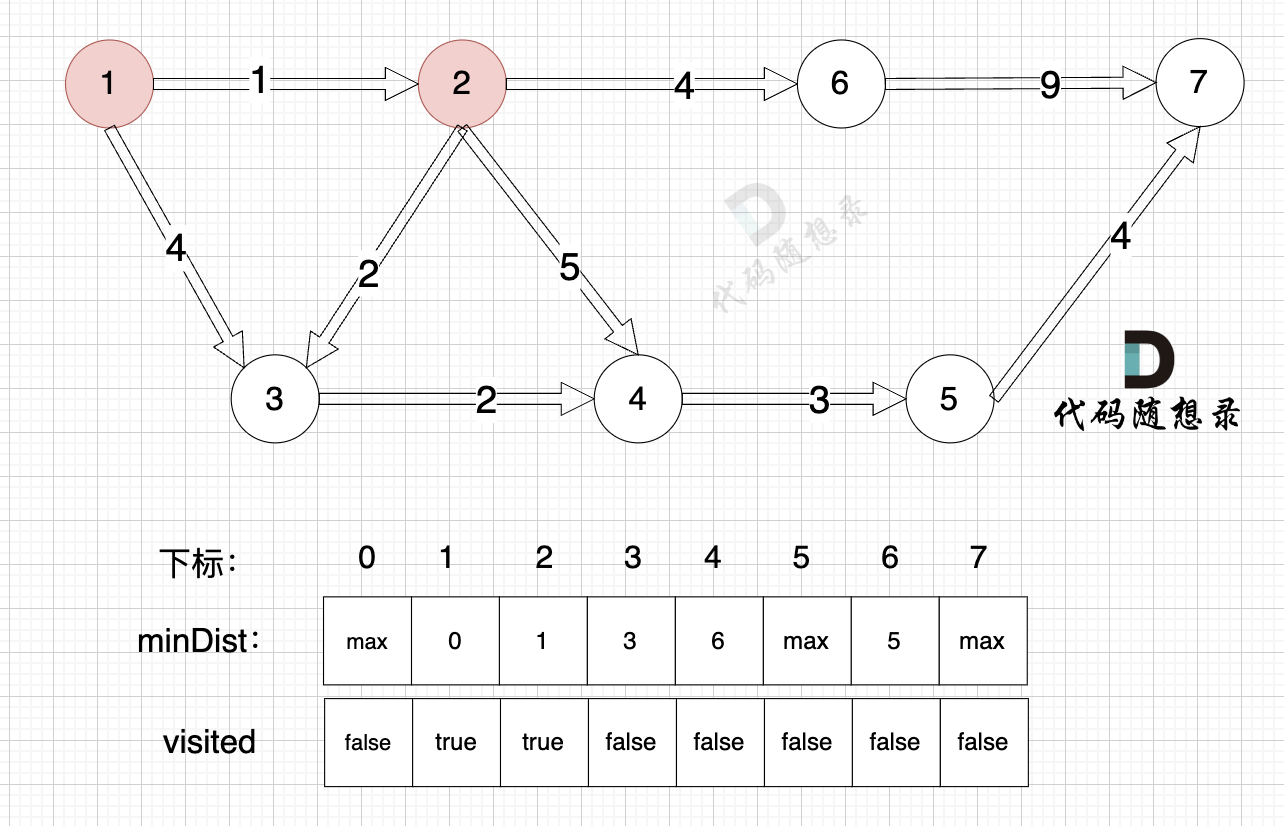
Update the `minDist` array, i.e., the distance from the source (node 1) to nodes 6, 3, and 4.

**Why update these nodes and not others?**

Because the source (node 1) can reach nodes 3, 4, and 6 via the already computed node 2.

Update the `minDist` array:

- The shortest distance from the source to node 6 is 5, which is less than the previous value of `minDist[6]`, which was `max`, so update `minDist[6] = 5`.
- The shortest distance from the source to node 3 is 3, which is less than the previous value of `minDist[3]`, which was 4, so update `minDist[3] = 3`.
- The shortest distance from the source to node 4 is 6, which is less than the previous value of `minDist[4]`, which was `max`, so update `minDist[4] = 6`.

-------------------

1. Choose the unvisited node closest to the start node.

Determine which nodes are closest to the source among unvisited ones, based on what?

Actually, look at the `minDist` array values. `minDist` records the closest distance from the source to all nodes, combining with the `visited` array to filter out visited nodes.

From the above diagram or from the `minDist` array, it is clear that among unvisited nodes, node 3 is closest to the source.

2. Mark this node as visited.

Mark node 3 as visited.

3. Update the distance to the source node for unvisited nodes (update the `minDist` array), as shown:

![Step 3](https://file1.kamacoder.com/i/algo/20240130120434.png) 

Due to the inclusion of node 3, the source can now connect to node 4 with a new path, so update the `minDist` array:

- The shortest distance from the source to node 4 is 5, which is less than the previous value of `minDist[4]`, which was 6, so update `minDist[4] = 5`.

------------------

1. Choose the unvisited node closest to the start node.

Node 4 and node 6, among unvisited nodes, are both closest to the source, both with a distance of 5 (`minDist[4] = 5`, `minDist[6] = 5`). Either node can be selected.

2. Mark this node as visited.

Mark node 4 as visited.

3. Update the distance to the source node for unvisited nodes (update the `minDist` array), as shown:

![Step 4](https://file1.kamacoder.com/i/algo/20240201105335.png) 

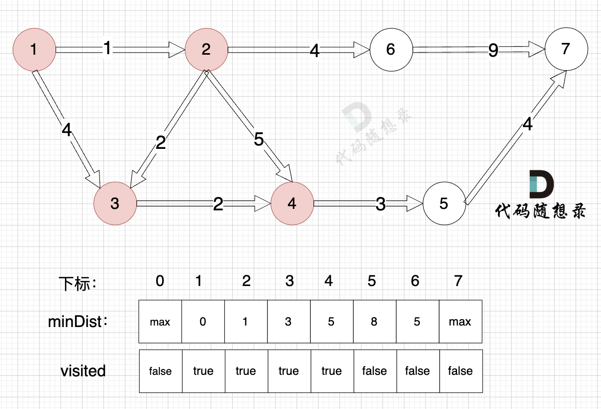
With node 4 included, the source can now connect to node 5, so update the `minDist` array:

- The shortest distance from the source to node 5 is 8, which is less than the previous value of `minDist[5]`, which was `max`, so update `minDist[5] = 8`.

--------------

1. Choose the unvisited node closest to the start node.

Node 6, among unvisited nodes, is closest to the source, with a distance of 5 (`minDist[6] = 5`). 

2. Mark this node as visited.

Mark node 6 as visited.

3. Update the distance to the source node for unvisited nodes (update the `minDist` array), as shown:

![Step 5](https://file1.kamacoder.com/i/algo/20240201110250.png)

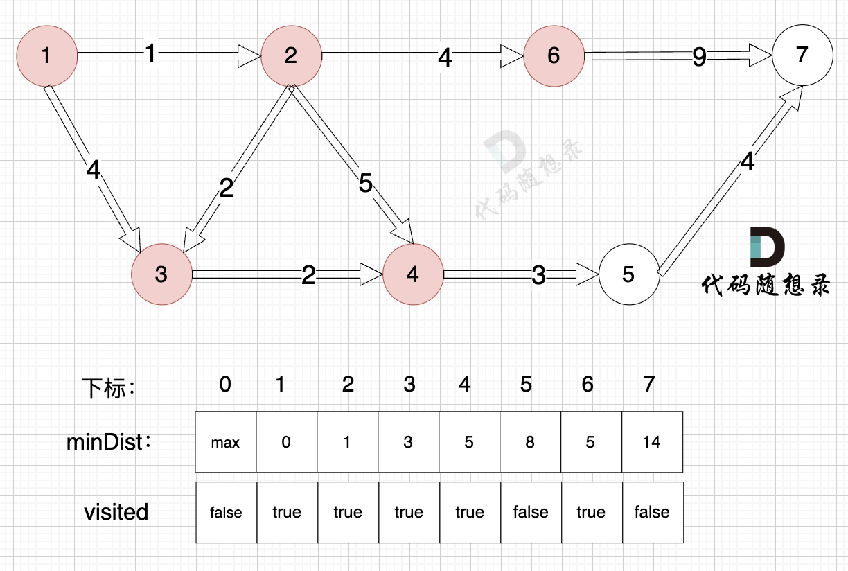
With node 6 included, the source can now connect to node 7, so update the `minDist` array:

- The shortest distance from the source to node 7 is 14, which is less than the previous value of `minDist[7]`, which was `max`, so update `minDist[7] = 14`.

-------------------

1. Choose the unvisited node closest to the start node.

Node 5, among unvisited nodes, is closest to the source, with a distance of 8 (`minDist[5] = 8`). 

2. Mark this node as visited.

Mark node 5 as visited.

3. Update the distance to the source node for unvisited nodes (update the `minDist` array), as shown:

![Step 6](https://file1.kamacoder.com/i/algo/20240201110651.png) 

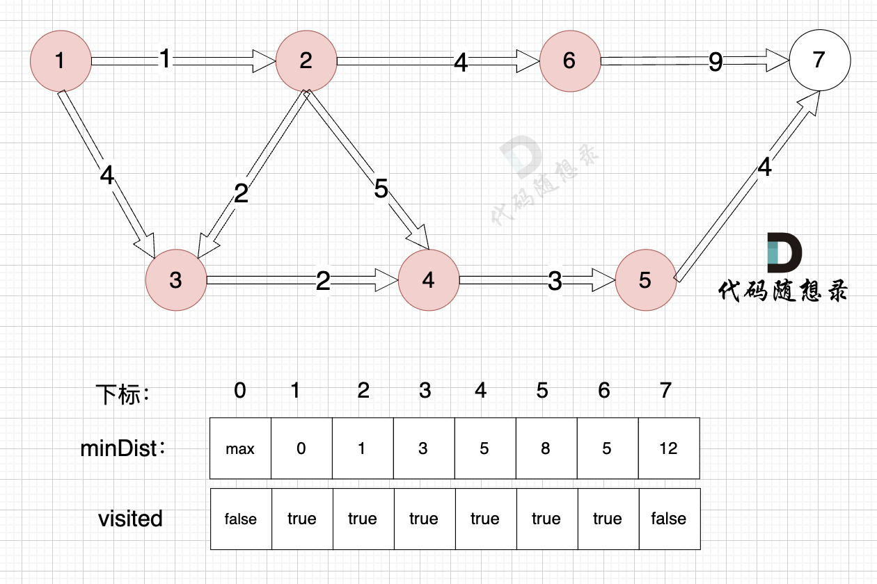
With node 5 included, the source can now connect to node 7 with a new path, so update the `minDist` array:

- The shortest distance from the source to node 7 is 12, which is less than the previous value of `minDist[7]`, which was 14, so update `minDist[7] = 12`.

-----------------

1. Choose the unvisited node closest to the start node.

Node 7 (the end node), among unvisited nodes, is closest to the source, with a distance of 12 (`minDist[7] = 12`).  

2. Mark this node as visited.

Mark node 7 as visited.

3. Update the distance to the source node for unvisited nodes (update the `minDist` array), as shown:

![Step 7](https://file1.kamacoder.com/i/algo/20240201110920.png)

Include node 7, but the distance from node 7 to node 7 is 0, so there's no need to update the `minDist` array.

--------------------

Finally, we need to find the distance from node 1 (the start node) to node 7 (the end node).

Let's recap the meaning of the `minDist` array: it records the shortest distance from any node to the source node.

Therefore, the shortest distance from the start (node 1) to the end (node 7) is `minDist[7]`. According to the previous explanation, `minDist[7] = 12`, and the shortest path from node 1 to node 7 has a weight of 12.

The path is shown in the diagram: 

![Shortest Path](https://file1.kamacoder.com/i/algo/20240201111352.png) 

In the explanation above, each step follows the Dijkstra Three Steps, and understanding these steps makes the code easy to understand. 

### Code Implementation

The code for this problem is as follows, with comments marking the three steps, and you can refer to the previous explanation to understand the following code:

```cpp
class Solution {
public:
    int networkDelayTime(vector<vector<int>>& times, int n, int k) {

        // Note: The 2D array provided in the problem is not the adjacency matrix
        // An adjacency matrix needs to be created to represent the graph
        // Because the numbering starts from 1, arrays will have size n+1
        vector<vector<int>> grid(n + 1, vector<int>(n + 1, INT_MAX));
        for(int i = 0; i < times.size(); i++){
            int p1 = times[i][0];
            int p2 = times[i][1];
            grid[p1][p2] = times[i][2];
        }

        // Stores the shortest distance from the source to each node
        std::vector<int> minDist(n + 1, INT_MAX);  

        // Records whether a vertex has been visited
        std::vector<bool> visited(n + 1, false); 

        minDist[k] = 0;  // Distance from the start to itself is 0
        for (int i = 1; i <= n; i++) {

            int minVal = INT_MAX;
            int cur = 1;

            // Traverse each node to find the unvisited node closest to the source
            for (int v = 1; v <= n; ++v) {
                if (!visited[v] && minDist[v] <= minVal) {
                    minVal = minDist[v];
                    cur = v;
                }
            }

            visited[cur] = true;  // Mark the vertex as visited

            for (int v = 1; v <= n; v++) {
                if (!visited[v] && grid[cur][v] != INT_MAX && minDist[cur] + grid[cur][v] < minDist[v]) {
                    minDist[v] = minDist[cur] + grid[cur][v];
                }
            }
        }
        // The time taken for the source to reach the farthest node, or the maximum of the shortest paths to all nodes
        int result = 0;
        for (int i = 1; i <= n; i++) {
            if (minDist[i] == INT_MAX) return -1; // No path
            result = max(minDist[i], result);
        }
        return result;
    }
};

• Time Complexity: O(n^2)
• Space Complexity: O(n^2)

Debugging Method

It is inevitable to encounter various issues when writing problems like this, so how do you determine whether your code has issues?

The best way is to log outputs, and for this problem, logging the minDist array can clearly reveal potential issues.

By selecting nodes in each step, whether the minDist array changes as expected, and whether it aligns with the logic I explained earlier.

For instance, for debugging purposes, the logging can be implemented as follows:

class Solution {
public:
    int networkDelayTime(vector<vector<int>>& times, int n, int k) {

        // Note: The 2D array provided in the problem is not the adjacency matrix
        // An adjacency matrix needs to be created to represent the graph
        // Because the numbering starts from 1, arrays will have size n+1
        vector<vector<int>> grid(n + 1, vector<int>(n + 1, INT_MAX));
        for(int i = 0; i < times.size(); i++){
            int p1 = times[i][0];
            int p2 = times[i][1];
            grid[p1][p2] = times[i][2];
        }

        // Stores the shortest distance from the source to each node
        std::vector<int> minDist(n + 1, INT_MAX);

        // Records whether a vertex has been visited
        std::vector<bool> visited(n + 1, false);

        minDist[k] = 0;  // Distance from the start to itself is 0
        for (int i = 1; i <= n; i++) {

            int minVal = INT_MAX;
            int cur = 1;

            // Traverse each node to find the unvisited node closest to the source
            for (int v = 1; v <= n; ++v) {
                if (!visited[v] && minDist[v] <= minVal) {
                    minVal = minDist[v];
                    cur = v;
                }
            }

            visited[cur] = true;  // Mark the vertex as visited

            for (int v = 1; v <= n; v++) {
                if (!visited[v] && grid[cur][v] != INT_MAX && minDist[cur] + grid[cur][v] < minDist[v]) {
                    minDist[v] = minDist[cur] + grid[cur][v];
                }
            }
            // Logging:
            cout << "select:" << cur << endl;
            for (int v = 1; v <= n; v++) cout <<  v << ":" << minDist[v] << " ";
            cout << endl << endl;
        }
        // The time taken for the source to reach the farthest node, or the maximum of the shortest paths to all nodes
        int result = 0;
        for (int i = 1; i <= n; i++) {
            if (minDist[i] == INT_MAX) return -1; // No path
            result = max(minDist[i], result);
        }
        return result;
    }
};

The logged result is as follows:

select:2
1:1 2:0 3:1 4:2147483647

select:3
1:1 2:0 3:1 4:2

select:1
1:1 2:0 3:1 4:2

select:4
1:1 2:0 3:1 4:2

The logs can be compared to the detailed process explained above, and each step's result aligns exactly with the prior explanation.

Thus, if your code has issues, using logs for debugging is the best method.

Occurrence of Negative Numbers

Would Dijkstra still work if the graph has negative edge weights?

Take a look at this graph: (with negative weights)

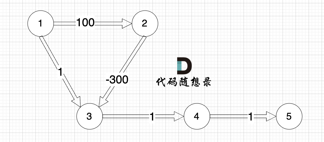
The shortest path from node 1 to node 5 should be node 1 -> node 2 -> node 3 -> node 4 -> node 5

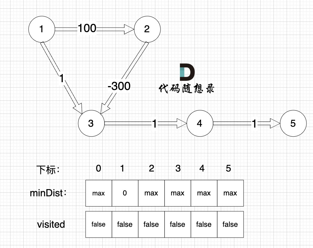
Let's see Dijkstra's calculated path for this problem using its three steps to simulate: (Refer to the Dijkstra simulation process above. Here, only critical processes like initialization are omitted.)

---

Initialization:

---

1. Choose the unvisited node closest to the start node.

The start node is closest to itself, with a distance of 0, and is unvisited.

2. Mark this node as visited.

Mark the start node as visited.

3. Update the distance to the source node for unvisited nodes (update the minDist array) as shown:

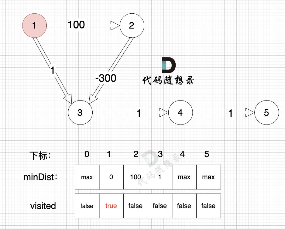
Update the minDist array, the shortest distance from the source (node 1) to nodes 2 and 3:

• The shortest distance from the source to node 2 is 100, less than the previous value of minDist[2], which was max, so update minDist[2] = 100.
• The shortest distance from the source to node 3 is 1, less than the previous value of minDist[3], which was max, so update minDist[4] = 1.

---

1. Choose the unvisited node closest to the start node.

The source node is closest to node 3, with a distance of 1, and is unvisited.

2. Mark this node as visited.

Mark node 3 as visited.

3. Update the distance to the source node for unvisited nodes (update the minDist array) as shown:

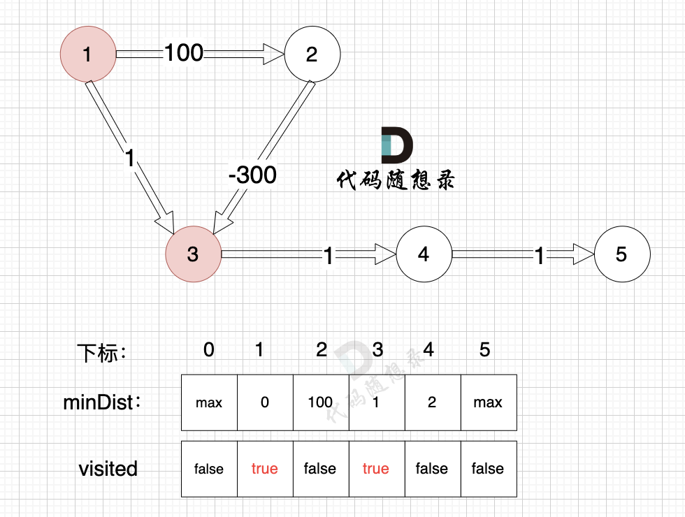
With node 3 included, the source can now connect node 4 using a new path, so update the minDist array:

• The shortest distance from the source to node 4 is 2, less than the previous value of minDist[4], which was max, so update minDist[4] = 2.

---

1. Choose the unvisited node closest to the start node.

The source node is closest to node 4 with a distance of 2, and is unvisited.

2. Mark this node as visited.

Mark node 4 as visited.

3. Update the distance to the source node for unvisited nodes (update the minDist array) as shown:

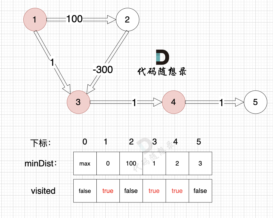
With node 4 included, the source can now connect node 5 using a new path, so update the minDist array:

• The shortest distance from the source to node 5 is 3, less than the previous value of minDist[5], which was max, so update minDist[5] = 5.

---

1. Choose the unvisited node closest to the start node.

Node 5, among unvisited nodes, is closest to the source, with a distance of 3 (minDist[5] = 3).

2. Mark this node as visited.

Mark node 5 as visited.

3. Update the distance to the source node for unvisited nodes (update the minDist array) as shown:

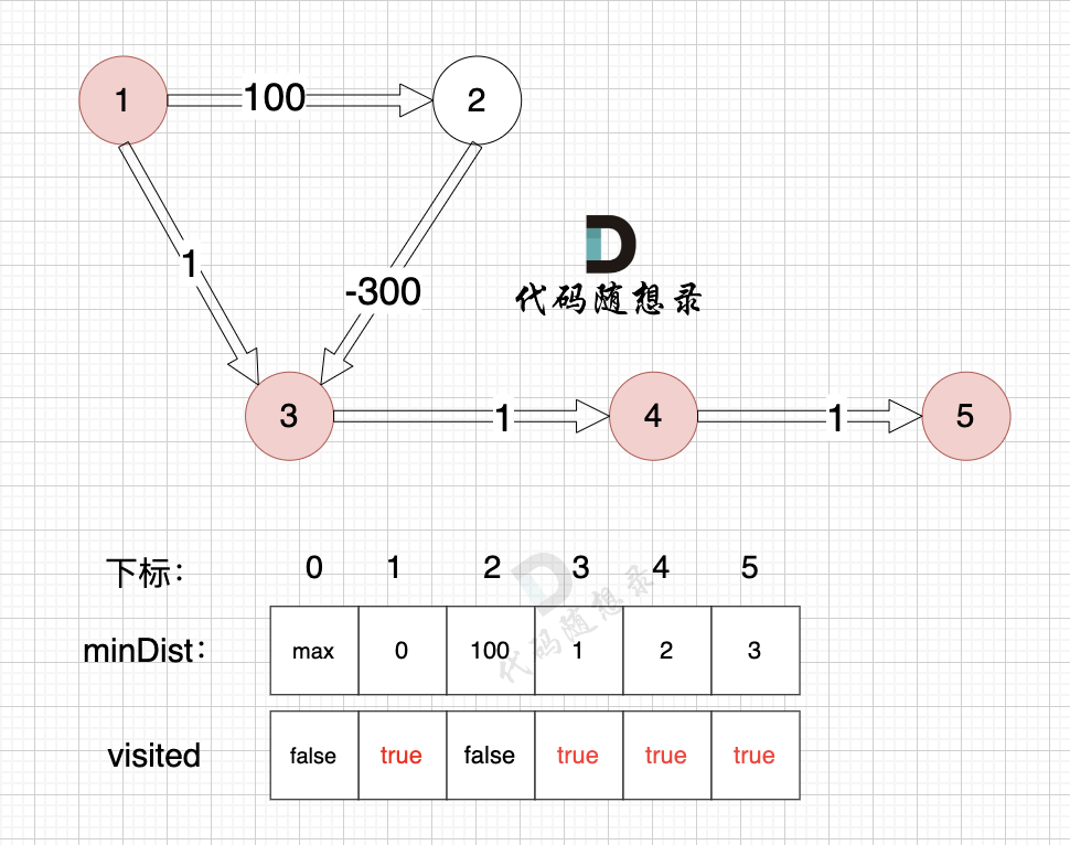
Node 5 is included, and it connects no other nodes, so there's no need to update the minDist array. Just mark node 5 as visited.

---

1. Choose the unvisited node closest to the start node.

Node 2, among unvisited nodes, is closest to the source, with a distance of 100 (minDist[2] = 100).

2. Mark this node as visited.

Mark node 2 as visited.

3. Update the distance to the source node for unvisited nodes (update the minDist array) as shown:

---

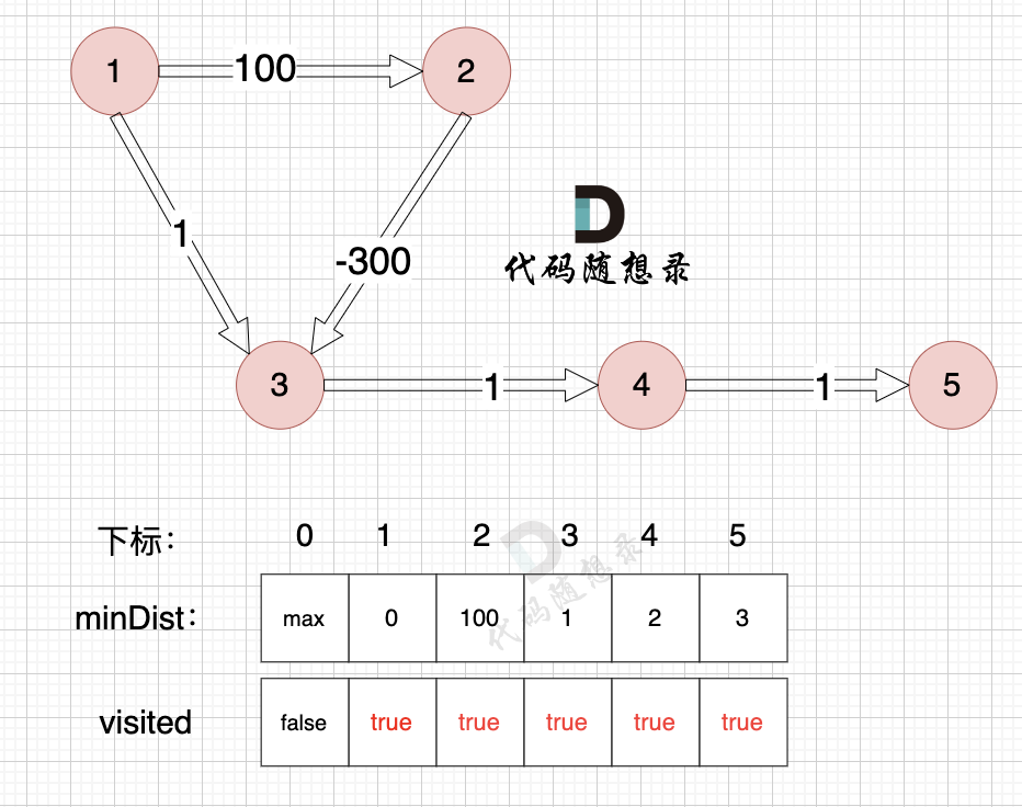
This concludes Dijkstra's simulation process. According to the final minDist array, the shortest path weight from node 1 to node 5 is 3: path 1 -> 3 -> 4 -> 5

Throughout this simulation, we see that despite not taking the negative weight path, it was because node 3 had already been visited by the time we reached node 2, blocking the discovery of the actual shortest path.

Some may think: Could we modify the code logic to allow visiting previously visited nodes?

However, allowing repeated visits to nodes may lead to an infinite loop. Is there a control mechanism to prevent this? (Feel free to try, practical exploration leads to the truth.)

When it comes to encountering negative weights, you may attempt to alter your Dijkstra approach continuously for a particular scenario, but ultimately, it is merely patching one hole while creating another. Modifying the logic to handle specific scenarios would only satisfy those particular cases but not a general solution.

For problems involving negative weights in graphs, the Floyd algorithm is better suited, which I will explain in detail later on.

Difference between Dijkstra and Prim's Algorithm

Again, it's essential to refer to the Prim's algorithm detailed discussion (opens new window) I provided beforehand; otherwise, you might not know what I'm referring to below.

You might notice Dijkstra's code structure closely resembles Prim's algorithm.

That's correct; the code is similar. The only real difference lies in the third step of the three steps: updating the minDist array.

Prim is concerned with finding the minimum spanning tree, while Dijkstra finds the shortest path to the source node.

Prim updates the minDist array like this:

for (int j = 1; j <= v; j++) {
    if (!isInTree[j] && grid[cur][j] < minDist[j]) {
        minDist[j] = grid[cur][j];
    }
}

In Prim's algorithm, the minDist represents the minimum distance from a node to the minimum spanning tree. Therefore, when a new current node cur is added, grid[cur][j] is invoked,

which determines the distance from the current node to node j.

Dijkstra's update of the minDist array looks like this:

for (int v = 1; v <= n; v++) {
    if (!visited[v] && grid[cur][v] != INT_MAX && minDist[cur] + grid[cur][v] < minDist[v]) {
        minDist[v] = minDist[cur] + grid[cur][v];
    }
}

In the minDist of Dijkstra's algorithm, a node's minimum distance is relative to the source node. Thus, adding a new current node cur involves (minDist[current]) to determine the shortest path to cur, plus the distance from cur to j (grid[cur][j]), to give the shortest path from the source to node j.

At this point, you might ponder over this question: Can Prim's algorithm have negative weights?

Of course!

Think for yourself and consider why?

Here's a hint: Prim’s algorithm needs to link nodes with minimum weights, but it doesn't relate to a single path.

Summary

In this article, we deeply discussed Dijkstra's algorithm and closely simulated its workflow.

Here I provided three steps of Dijkstra to help you understand the algorithm. This will assist in writing a framework and easy debugging even if, after a while, you might have forgotten some of Dijkstra's details.

For graph algorithms, the code is usually extensive and unlikely to pass on the first submission. Understanding how to debug is crucial.

That's why I dedicated a portion of this article to explaining my debugging methods.

This problem requires finding the minimum path sum, and at the same time, we're expected to understand how to print the shortest path.

I addressed the situation with negative weights in detail. By illustrating step-by-step Dijkstra's solution with negative weights, it helps identify where the underlying problems might lie.

If I'd just said, because previously visited nodes aren't revisited, it misses the actual shortest path, you would likely not grasp what I meant.

Finally, I also explained the similarities and differences between Dijkstra and Prim's algorithms. I chose to explain Prim's algorithm before Dijkstra's to provide clarity, since understanding both algorithms' similarities aids deeper learning.

Rather than isolating Dijkstra after learning it, finding relationships between algorithms will foster deeper thinking and more thorough mastery.

I have written considerably here, which only covers the basic version of Dijkstra’s algorithm. For heap-optimized Dijkstra, I will provide detailed explanations in the next article.

Dijkstra's Algorithm with Heap Optimization

In this article, we will discuss the heap optimization version of Dijkstra. Be sure to read my explanation of the basic version of Dijkstra first; otherwise, certain parts of this article may be unclear.

In the previous article, we discussed the basic version of Dijkstra's algorithm, which has a time complexity of (O(n^2)). Notice that its time complexity is only related to (n) (number of nodes).

When (n) is very large, we can consider other perspectives to improve performance.

In the discussion of minimum spanning trees, we talked about two algorithms: Prim's Algorithm (opens new window) (finding the minimum spanning tree from the node perspective) and Kruskal's Algorithm (opens new window) (finding it from the edge perspective).

Similarly, when (n) (number of nodes) is very large and the number of edges is also substantial (dense graph), the initial solution works well.

However, when (n) (number of nodes) is significant, and the number of edges is small (sparse graph), is it possible to shift the perspective to edges to find the shortest path?

After all, there are fewer edges.

Some readers might think: Can there really be any graphs where nodes are numerous but edges are few?

Don't forget, there's no requirement for nodes to be interconnected by edges, for instance, a graph with ten thousand nodes and only one edge—this is still a valid graph.

Understanding the background, let's explore the solution.

Graph Storage

First, let's discuss graph storage.

There are two mainstream ways to store a graph: adjacency matrix and adjacency list.

Adjacency Matrix

An adjacency matrix uses a two-dimensional array to represent the graph structure. It captures the graph from the nodes' perspective by using a 2D array whose size corresponds to the number of nodes.

For example: grid[2][5] = 6 represents a directed graph where node 2 points to node 5 with a weight of 6. It could signify, in the context of the problem, a distance of 6 or a weight consumption of 6, etc.

For an undirected graph: grid[2][5] = 6, grid[5][2] = 6 indicates nodes 2 and 5 are mutually connected with a weight of 6.

As illustrated:

An (n) (number of nodes) equals 8 graph will require (8 \times 8) space. The matrix holds, for example, one bidirectional edge: grid[2][5] = 6, grid[5][2] = 6.

This data structure (adjacency matrix) will, in cases of sparse graphs with many nodes, cause space inefficiency by occupying unnecessarily large 2D array space.

Additionally, searching for node connections demands a complete traversal of the matrix, resulting in a time complexity of (n \times n), causing time inefficiency.

Advantages of adjacency matrices:

• Simple and easy to comprehend expressiveness.
• Checking the existence of an edge between any two vertices is efficient.
• Suitable for dense graphs. In graphs where edge count approximates the square of the vertex count, adjacency matrix representation offers high space efficiency.

Disadvantages:

• Space waste for sparse graphs due to large space allocations, and time waste traversing the (n \times n) matrix during edge checks.

Adjacency List

An adjacency list uses an array plus a linked list to represent the graph. Adjacency lists record graphs in the context of edge counts, requesting chain nodes corresponding to the number of edges.

Constructing adjacency lists, illustrated:

This demonstrates:

• Node 1 points to nodes 3 and 5.
• Node 2 points to nodes 4, 3, and 5.
• Node 3 points to node 4.
• Node 4 points to node 1.

The adjacency list requests chain nodes based on the number of edges.

The graph structure uses arrays and linked lists, as visualized above, to demonstrate node linkage.

Advantages of adjacency lists:

• High space utilization for storing sparse graphs as only edges are recorded.
• Relative simplicity in traversing node connections.

Disadvantages:

• Lower efficiency in examining connectivities between any two nodes, operation time complexity being (O(V)) where (V) represents nodes connected to a given node.
• Relative complexity in implementation, demanding greater ease of comprehension.

Graph Storage for This Problem

Now, let's continue analyzing this problem from the perspective of a sparse graph.

In the basic version of the solution, we mentioned three steps:

1. Step one: Choose the unvisited node closest to the start node.
2. Step two: Mark this closest node as visited.
3. Step three: Update the distance to the source node for unvisited nodes (update minDist array).

In the first version of the code, these three steps are within a for loop, but why?

Since we solved it from the node perspective.

The traversal of edge costs in the first step (selecting an unvisited node closest to the start) inherently calls for traversing minDist to find the closest unvisited node.

Simultaneously, we need to traverse all unvisited nodes, requiring two nested for loops from the node angle for the basic version. Here's the code: (note code comments marking the purpose of the loops)

for (int i = 1; i <= n; i++) { // Traverse every node, in the first loop.

    int minVal = INT_MAX;
    int cur = 1;

    // 1. Choose the nearest unvisited node to the source
    for (int v = 1; v <= n; ++v) { // Second loop   
        if (!visited[v] && minDist[v] < minVal) {
            minVal = minDist[v];
            cur = v;
        }
    }

    visited[cur] = true;  // Mark that the node has been visited.

    // 3. Third step, update the minimum distance array for unvisited nodes.
    for (int v = 1; v <= n; v++) { 
        if (!visited[v] && grid[cur][v] != INT_MAX && minDist[cur] + grid[cur][v] < minDist[v]) {
            minDist[v] = minDist[cur] + grid[cur][v];
        }
    }

}

When considering the graph from the angle of edge prominence, the first step in Dijkstra's three-step approach (selecting the node nearest to the source that remains unvisited) foregoes the need for looping through all nodes.

Instead, by inputting edges (with weights) into a min-heap, they can automatically sort the edges, allowing for quick access to the edge leading to the node nearest the source each time.

Thus, by sidestepping the need for a double for loop to pinpoint the nearest node.

With an understanding of the basic concept, let's examine the code's execution.

First, let's see how adjacency lists are implemented as they pose the initial hurdle for many readers unfamiliar with the representation.

To represent the adjacency list (array+linked list) of size n+1 in C++ with vector and list, the following code is used:

vector<list<int>> grid(n + 1);

Many users are unsure about defining the structure and expressing the adjacency list. Here’s how it’s illustrated:

This diagram signifies:

• Node 1 points to nodes 3 and 5.
• Node 2 points to nodes 4, 3, and 5.
• Node 3 points to node 4.
• Node 4 points to node 1.

Assuming that the graph edges have no weights, however, to solve this problem, we must record weights—where should they be?

Consequently, instead of using int, a key-value pair to store two integers is necessary because the problem's graph edges possess weights:

vector<list<pair<int,int>>> grid(n + 1);

To illustrate how this code represents weighted graphs:

• Node 1 points to node 3 with a weight of 1
• Node 1 points to node 5 with a weight of 2
• Node 2 points to node 4 with a weight of 7
• Node 2 points to node 3 with a weight of 6
• Node 2 points to node 5 with a weight of 3
• Node 3 points to node 4 with a weight of 3
• Node 4 points to node 1 with a weight of 10

This effectively captures weights within the graph structure.

To enhance clarity and readability, instead of directly using pair<int, int>, defining a class helps manage those values clearly, preventing confusion.

The class (or structure) would be defined as:

struct Edge {
    int to;  // Adjacent vertex
    int val; // Edge's weight

    Edge(int t, int w): to(t), val(w) {}  // Constructor
};

The class contains named member variables, avoiding ambiguity in understanding the two integers’ purposes.

Thus, this problem employs an adjacency list with the following structure:

struct Edge {
    int to;  // Adjacent vertex
    int val; // Edge's weight

    Edge(int t, int w): to(t), val(w) {}  // Constructor
};

vector<list<Edge>> grid(n + 1); // Adjacency list

(Referencing the adjacency list code for how this is expressed in the subsequent explanation)

Heap Optimization Details

Conceptually, exact replication of Dijkstra's three steps:

1. Step one: Choose the unvisited node closest to the start node.
2. Step two: Mark this closest node as visited.
3. Step three: Update the distance to the source node for unvisited nodes (update the minDist array).

However, before traversing nodes to traverse edges as the basic version does within two nested loops, sort new connecting edges with a heap, leading directly to nodes closest to the source.

How do we manage this sorting within step one of Dijkstra, efficiently selecting the nearest unvisited node?

By employing a min-heap, allowing edges' weights to determine their order, we achieve the optimal selection with a heap.

In C++, implementing a min-heap uses a priority_queue, like this:

// Min-heap
class mycomparison {
public:
    bool operator()(const pair<int, int>& lhs, const pair<int, int>& rhs) {
        return lhs.second > rhs.second;
    }
};
// Priority queue stores pair<node number, weight to that node from source>
priority_queue<pair<int, int>, vector<pair<int, int>>, mycomparison> pq;

(The pair<int, int> stores the weight from the source to nodes as the second int for the min-heap sorting)

With a min-heap automating edge weight sorting, we extract the top of the heap directly, showing the node nearest to the source.

Step one of Dijkstra's Three Steps no longer requires a for loop:

// pair<node number, weight to that node from source>
pair<int, int> cur = pq.top(); pq.pop();

The second step, marking the retrieved node as visited, operates similarly to basic Dijkstra:

// 2. Now, mark that nearest node visited
visited[cur.first] = true;

(cur.first is the node number retrieved from pair<int, int>, which pairs nodes and weights)

The third step, "updating the distance to the source node for unvisited nodes", follows the familiar logic of basic Dijkstra.

However, this poses a considerable challenge for many if unfamiliar with:

• Not understanding Dijkstra's proposal thoroughly.
• Unacquaintance with how adjacency lists work.

Let's revisit the basic Dijkstra code and concepts (if you haven't seen the basic version I discussed before, this will be confusing):

// 3. Now, update the distances for unvisited nodes to the source node
for (int v = 1; v <= n; v++) {
    if (!visited[v] && grid[cur][v] != INT_MAX && minDist[cur] + grid[cur][v] < minDist[v]) {
        minDist[v] = minDist[cur] + grid[cur][v];
    }
}

The loop's purpose? Discovering nodes cur is connected to involves looping through every node whenever using adjacency matrices.

In contrast, within an adjacency list, we optimize this by readily knowing what nodes a specific node is connected to.

Recall the construction of adjacency lists (array+list):

If the node being added, cur, is node 2, then grid[2] equates to the entire second row of chains from the graph for node processing (the construction of the grid array is detailed in "Graph Storage" above).

The loop methodology to fulfill connections using C++ follows:

for (Edge edge : grid[cur.first]) 

(If confused about what Edge refers to, refer to “Graph Storage” for adjacency list explanation)

cur.first refers to the current node number, understanding it in light of pair construction: pair<node number, weight to that node from source>.

Proceed to distance updates for unvisited nodes. Code implementation aligns with basic Dijkstra:

// 3. Now, update the distance to the source node for unvisited nodes (i.e., `minDist` array)
for (Edge edge : grid[cur.first]) {  // Traverse nodes `cur` points to, as edges `edge`.
    // Here: `edge.to` is the node `cur` points to; this edge has weight `edge.val`
    if (!visited[edge.to] && minDist[cur.first] + edge.val < minDist[edge.to]) {  // Time for `minDist` updating
        minDist[edge.to] = minDist[cur.first] + edge.val;
        pq.push(pair<int, int>(edge.to, minDist[edge.to]));
    }
}

Why does this divergence between adjacency lists and matrices occur? Likely, lesser understanding of adjacency list representation amongst some.

Within the code, the current node cur connecting to edge.to has a connection weight of edge.val. Ensure edge.to remains unvisited, marked with !visited[edge.to]. The combined minimum distance to the cur node and from cur to edge.to, (minDist[cur.first] + edge.val), gives a new degree of connectivity and updates the distance system as follows should it outscore existing minDist[edge.to].

This yields:

if (!visited[edge.to] && minDist[cur.first] + edge.val < minDist[edge.to]) {  // Update the `minDist` structure
    minDist[edge.to] = minDist[cur.first] + edge.val;
    pq.push(pair<int, int>(edge.to, minDist[edge.to])); // With `cur`'s addition, source gains new applicable connections
}

• By introducing cur, new dynamic routes take form via unexploited adjacent nodes. In turn, include these innovative paths within the priority queue.

These codes, operationally or conceptually, precisely mirror basic Dijkstra's methodology—distinguished only by the disparate adjacency list encoding and prioritization queue application in edge sorting.

Complete Code Implementation

Here is the full code for heap optimization version Dijkstra:

class Solution {
public:
    // Min-heap
    class mycomparison {
    public:
        bool operator()(const pair<int, int>& lhs, const pair<int, int>& rhs) {
            return lhs.second > rhs.second;
        }
    };
    // Define a structure for edges featuring weights
    struct Edge {
        int to;  // Adjacent vertex
        int val; // Edge's weight

        Edge(int t, int w): to(t), val(w) {}  // Constructor
    };
    int networkDelayTime(vector<vector<int>>& times, int n, int k) {

        std::vector<std::list<Edge>> grid(n + 1);
        for(int i = 0; i < times.size(); i++){
            int p1 = times[i][0];
            int p2 = times[i][1];
            // p1 pointing to p2, weight is times[i][2]
            grid[p1].push_back(Edge(p2, times[i][2]));
        }

        // Store the shortest distance from the source node to each node
        std::vector<int> minDist(n + 1, INT_MAX);

        // Record whether a vertex has been visited
        std::vector<bool> visited(n + 1, false);

        // Priority queue storing pair<node, distance from the source>
        priority_queue<pair<int, int>, vector<pair<int, int>>, mycomparison> pq;

        pq.push(pair<int, int>(k, 0));
        minDist[k] = 0;  // This should not be forgotten

        while (!pq.empty()) {
            // <node, distance from the source>
            // 1. Choose which node is closest to the source and unvisited (achieved using priority queue)
            pair<int, int> cur = pq.top(); pq.pop();

            if (visited[cur.first]) continue;  // Skip if already visited

            // 2. Now, mark that nearest node visited
            visited[cur.first] = true;

            // 3. Third step, update `minDist` for unvisited nodes
            for (Edge edge : grid[cur.first]) { // Traverse nodes `cur` points to, as edges `edge`
                // The node `cur` points to is `edge.to`, and this edge's weight is `edge.val`
                if (!visited[edge.to] && minDist[cur.first] + edge.val < minDist[edge.to]) { // Performing `minDist` updating
                    minDist[edge.to] = minDist[cur.first] + edge.val;
                    pq.push(pair<int, int>(edge.to, minDist[edge.to])); // `cur` joining enables new paths pointing to the source
                }
            }

        }
        // Now, `result` records the longest short paths leading to the rest across the graph
        int result = 0;
        for (int i = 1; i <= n; i++) {
            if (minDist[i] == INT_MAX) return -1;  // No path exists
            result = max(minDist[i], result);
        }
        return result;
    }
};

• Time Complexity: (O(E\log{E})) , where (E) is the number of edges
• Space Complexity: (O(N + E)), where (N) is the number of nodes

Heap optimization time complexity primarily drives edge quantity while factoring out the count of nodes. Each element in the queue represents an edge.

Analyzing the loop within while (! pq.empty()), the entire dataset processes into the queue once across all edges, with corresponding edge removals.

Edges insert once yielding a complexity of (O(E)), while (! pq.empty()) where queue operations employ a heap with removal time complexity as (O (\log{E})), which stems from heap scalar operations.

(The structuring is identical whether ordering occurs during edge additions or threshold retrievals, providing consistent (O({E})) total complexity. Importantly, the heap lacks residual buildup, so queued and removed elements are one-to-one.)

Thus, (O({E}\log{E})) arises for optimized algorithmic time complexity.

Online resources suggesting node inclusion in analysis often err; consider an extreme where n amounts to (10000) linked by a single edge; code process comprehension traces work iterations as once only.

Hence, algorithmic time complexity remains node-independent.

Space requirement complexity arises from adjacency list's hybrid structure of array plus linked list spanning (N) plus (E) set apart edges resulting in complexity of (N + E).

Expansion

Still, there are discussions regarding possibilities for heap optimizing Dijkstra while still utilizing adjacency matrices, is that possible?

Certainly possible.

However, considering current sparsity, opting for advanced adjacency matrix models had squandered potential optimization. Efficient algorithms implementing inefficient data structures likely dilute performance gain.

If confusion persists regarding adjacency list preference, expanded comprehension around "Graph Storage" previously elaborates.

Here is an adjacency matrix versioned Dijkstra heap optimization code included:

class Solution {
public:
    // Min-heap (orders arrays based on `<k ,v>` as `v` in ascending order )
    class mycomparison {
    public:
        bool operator()(const pair<int, int>& lhs, const pair<int, int>& rhs) {
            return lhs.second > rhs.second;
        }
    };
    int networkDelayTime(vector<vector<int>>& times, int n, int k) {

        // Note: The provided 2D arrays from the problem are not adjacency matrices
        // The graph uses adjacency matrices for graph representation
        // Nodes numbered from 1, hence arrays extend from 1 to n+1
        vector<vector<int>> grid(n + 1, vector<int>(n + 1, INT_MAX));
        for(int i = 0; i < times.size(); i++){
            int p1 = times[i][0];
            int p2 = times[i][1];
            grid[p1][p2] = times[i][2];
        }

        // Store minimum distances from the source for each node
        std::vector<int> minDist(n + 1, INT_MAX);

        // Log whether nodes receive visitation
        std::vector<bool> visited(n + 1, false);

        // Priority queues to preserve `pair<node, source - node distance>` style
        priority_queue<pair<int, int>, vector<pair<int, int>>, mycomparison> pq;

        pq.push(pair<int, int>(k, 0));
        minDist[k] = 0; 

        while (!pq.empty()) {
            // `<node, source - node distance>`
            // 1. Select the nearest unvisited node to the source 
            pair<int, int> cur = pq.top(); pq.pop();

            if (visited[cur.first]) continue;

            // 2. Logging has occurred for visited vertex
            visited[cur.first] = true;

            // 3. Subsequent steps; update minimum distance markings for unvisited nodes (`minDist`)
            // Traversal of nodes applicable via `cur`
            for (int j = 1; j <= n; j++) {
                if (!visited[j] && grid[cur.first][j] != INT_MAX && (minDist[cur.first] + grid[cur.first][j] < minDist[j])) {
                    minDist[j] = minDist[cur.first] + grid[cur.first][j];
                    pq.push(pair<int, int>(j, minDist[j]));
                }
            }
        }

        // `result` logs for most distant point across nodes, thus signaling maximum among reachable shortest paths 
        int result = 0;
        for (int i = 1; i <= n; i++) {
            if (minDist[i] == INT_MAX) return -1;// No available path
            result = max(minDist[i], result);
        }
        return result;
    }
};

• Time Complexity: (O(E \times (N + \log{E}))) , where (E) is the edge count, and (N) is the node count
• Space Complexity: (O(\log {(N^2)})

Inclusion of while (! pq.empty()) structure signifies time complexity with (E), and nested (while) executes (O(\log{E})) complexity through priority queue procedures, while incorporating a for loop spanning (N).

Altogether averaging (O(E \times (N+\log{E}))) potentially responding to concerns of node figures.

This accounts for every conceivable code path as incalculable minDist inefficiencies captured via intermediate.

Summary

When learning an optimal strategy, initially understanding what's improved and the challenges it confronts is crucial.

Therefore, within this article, I anticipate providing context around why heap optimization stood necessary.

An analogous execution follows Dijkstra’s overall model in subsequent optimals, yet with additional contrasting and distinct phases to surface further clarity.

Primary misconception arises among inexperienced readers around central theoretical underlying validity within adjacency lists—the foremost challenge dealt in an introductory piece broadened utilization.

Covered also is adjacency list-efficient processing with a developed code logic.

Therefore, for heap optimization benefits are manifestly illustrated and tailored alongside simple logic.

Prioritization queue-based node processing guarantees executional efficiency gains translate towards strategic edge orientation supplemented by sorting-driven expediency.

The article features unconventional cases for adjacency matrix-oriented assessments, dovetailing complete alternative community analysis.

Overall, gets resolved balance between troubleshooting execution compatibilities with optimizing redundancies.